Categories
Offsites

LOLNeRF: Learn from One Look

An important aspect of human vision is our ability to comprehend 3D shape from the 2D images we observe. Achieving this kind of understanding with computer vision systems has been a fundamental challenge in the field. Many successful approaches rely on multi-view data, where two or more images of the same scene are available from different perspectives, which makes it much easier to infer the 3D shape of objects in the images.

There are, however, many situations where it would be useful to know 3D structure from a single image, but this problem is generally difficult or impossible to solve. For example, it isn’t necessarily possible to tell the difference between an image of an actual beach and an image of a flat poster of the same beach. However it is possible to estimate 3D structure based on what kind of 3D objects occur commonly and what similar structures look like from different perspectives.

In “LOLNeRF: Learn from One Look”, presented at CVPR 2022, we propose a framework that learns to model 3D structure and appearance from collections of single-view images. LOLNeRF learns the typical 3D structure of a class of objects, such as cars, human faces or cats, but only from single views of any one object, never the same object twice. We build our approach by combining Generative Latent Optimization (GLO) and neural radiance fields (NeRF) to achieve state-of-the-art results for novel view synthesis and competitive results for depth estimation.

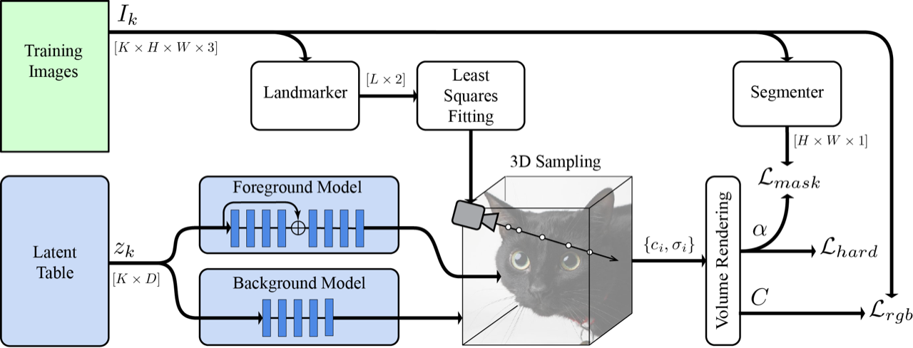
We learn a 3D object model by reconstructing a large collection of single-view images using a neural network conditioned on latent vectors, z (left). This allows for a 3D model to be lifted from the image, and rendered from novel viewpoints. Holding the camera fixed, we can interpolate or sample novel identities (right).

Combining GLO and NeRF
GLO is a general method that learns to reconstruct a dataset (such as a set of 2D images) by co-learning a neural network (decoder) and table of codes (latents) that is also an input to the decoder. Each of these latent codes re-creates a single element (such as an image) from the dataset. Because the latent codes have fewer dimensions than the data elements themselves, the network is forced to generalize, learning common structure in the data (such as the general shape of dog snouts).

NeRF is a technique that is very good at reconstructing a static 3D object from 2D images. It represents an object with a neural network that outputs color and density for each point in 3D space. Color and density values are accumulated along rays, one ray for each pixel in a 2D image. These are then combined using standard computer graphics volume rendering to compute a final pixel color. Importantly, all these operations are differentiable, allowing for end-to-end supervision. By enforcing that each rendered pixel (of the 3D representation) matches the color of ground truth (2D) pixels, the neural network creates a 3D representation that can be rendered from any viewpoint.

We combine NeRF with GLO by assigning each object a latent code and concatenating it with standard NeRF inputs, giving it the ability to reconstruct multiple objects. Following GLO, we co-optimize these latent codes along with network weights during training to reconstruct the input images. Unlike standard NeRF, which requires multiple views of the same object, we supervise our method with only single views of any one object (but multiple examples of that type of object). Because NeRF is inherently 3D, we can then render the object from arbitrary viewpoints. Combining NeRF with GLO gives it the ability to learn common 3D structure across instances from only single views while still retaining the ability to recreate specific instances of the dataset.

Camera Estimation
In order for NeRF to work, it needs to know the exact camera location, relative to the object, for each image. Unless this was measured when the image was taken, it is generally unknown. Instead, we use the MediaPipe Face Mesh to extract five landmark locations from the images. Each of these 2D predictions correspond to a semantically consistent point on the object (e.g., the tip of the nose or corners of the eyes). We can then derive a set of canonical 3D locations for the semantic points, along with estimates of the camera poses for each image, such that the projection of the canonical points into the images is as consistent as possible with the 2D landmarks.

We train a per-image table of latent codes alongside a NeRF model. Output is subject to per-ray RGB, mask and hardness losses. Cameras are derived from a fit of predicted landmarks to canonical 3D keypoints.
Example MediaPipe landmarks and segmentation masks (images from CelebA).

Hard Surface and Mask Losses
Standard NeRF is effective for accurately reproducing the images, but in our single-view case, it tends to produce images that look blurry when viewed off-axis. To address this, we introduce a novel hard surface loss, which encourages the density to adopt sharp transitions from exterior to interior regions, reducing blurring. This essentially tells the network to create “solid” surfaces, and not semi-transparent ones like clouds.

We also obtained better results by splitting the network into separate foreground and background networks. We supervised this separation with a mask from the MediaPipe Selfie Segmenter and a loss to encourage network specialization. This allows the foreground network to specialize only on the object of interest, and not get “distracted” by the background, increasing its quality.

Results
We surprisingly found that fitting only five key points gave accurate enough camera estimates to train a model for cats, dogs, or human faces. This means that given only a single view of your beloved cats Schnitzel, Widget and friends, you can create a new image from any other angle.
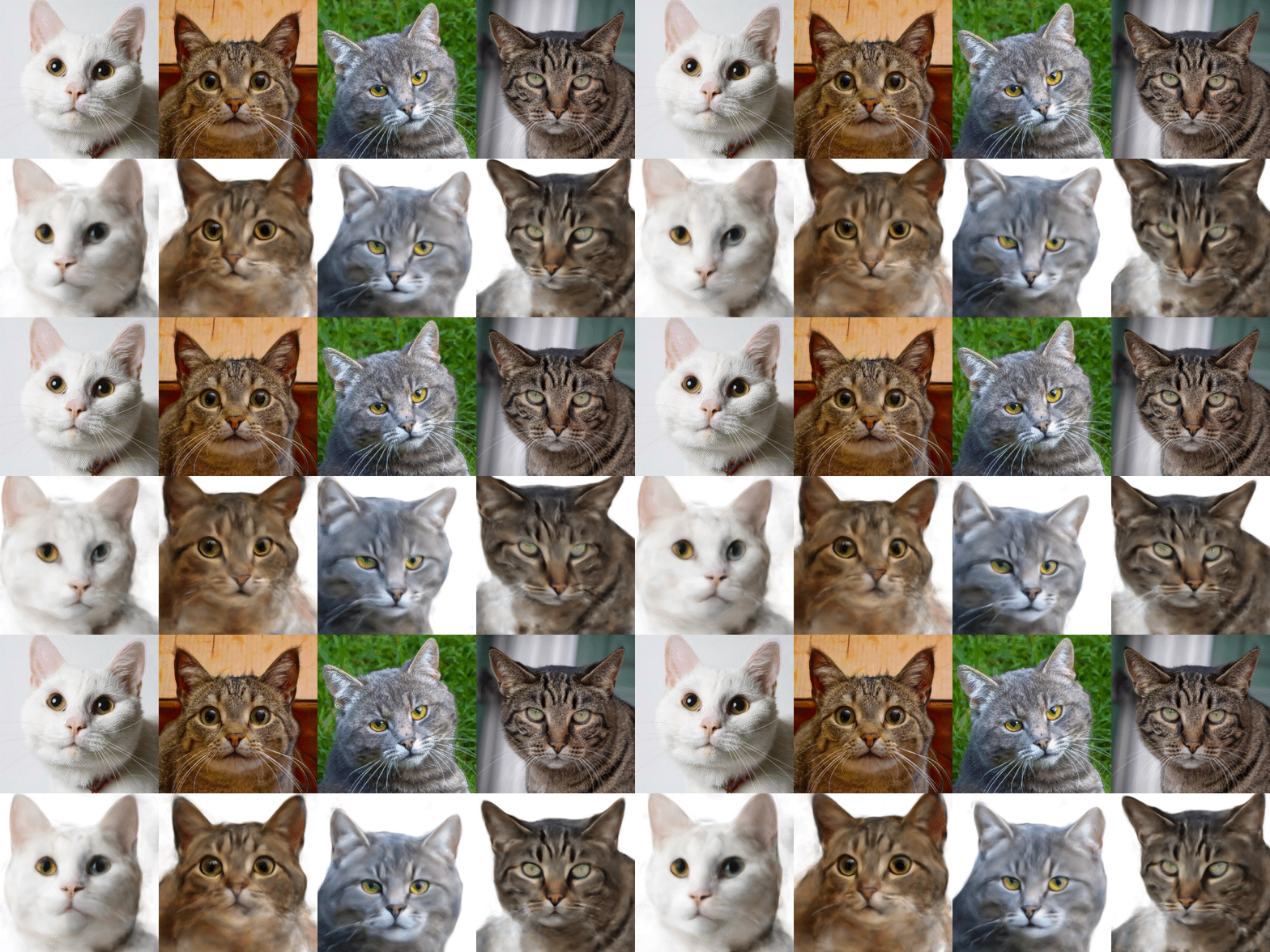
Top: example cat images from AFHQ. Bottom: A synthesis of novel 3D views created by LOLNeRF.

Conclusion
We’ve developed a technique that is effective at discovering 3D structure from single 2D images. We see great potential in LOLNeRF for a variety of applications and are currently investigating potential use-cases.

Interpolation of feline identities from linear interpolation of learned latent codes for different examples in AFHQ.

Code Release
We acknowledge the potential for misuse and importance of acting responsibly. To that end, we will only release the code for reproducibility purposes, but will not release any trained generative models.

Acknowledgements
We would like to thank Andrea Tagliasacchi, Kwang Moo Yi, Viral Carpenter, David Fleet, Danica Matthews, Florian Schroff, Hartwig Adam and Dmitry Lagun for continuous help in building this technology.

Categories
Misc

Get up to Speed: Five Reasons Not to Miss NVIDIA CEO Jensen Huang’s GTC Keynote Sept. 20

Think fast. Enterprise AI, new gaming technology, the metaverse and the 3D internet, and advanced AI technologies tailored to just about every industry are all coming your way. NVIDIA founder and CEO Jensen Huang’s keynote at NVIDIA GTC on Tuesday, Sept. 20, is the best way to get ahead of all these trends. NVIDIA’s virtual Read article >

The post Get up to Speed: Five Reasons Not to Miss NVIDIA CEO Jensen Huang’s GTC Keynote Sept. 20 appeared first on NVIDIA Blog.

Categories
Misc

AI on the Stars: Hyperrealistic Avatars Propel Startup to ‘America’s Got Talent’ Finals

More than 6 million pairs of eyes will be on real-time AI avatar technology in this week’s finale of America’s Got Talent — currently the second-most popular primetime TV show in the U.S.. Metaphysic, a member of the NVIDIA Inception global network of technology startups, is one of 11 acts competing for $1 million and Read article >

The post AI on the Stars: Hyperrealistic Avatars Propel Startup to ‘America’s Got Talent’ Finals appeared first on NVIDIA Blog.

Categories
Misc

Using Vulkan SC for Safety-Critical Graphics and Real-time GPU Processing

GPU-accelerated processing is vital to many automotive and embedded systems. Safety-critical and real-time applications have different requirements and…
GPU-accelerated processing is vital to many automotive and embedded systems. Safety-critical and real-time applications have different requirements and deployment priorities than consumer applications, but they often are developed using GPU APIs that have been primarily designed for use in games.

Vulkan SC (Safety Critical) is a newly released open standard to streamline the use of GPUs in markets where functional safety and hitch-free performance are essential.

NVIDIA helped lead the creation of the Vulkan SC 1.0 API and is now shipping production drivers on its NVIDIA DRIVE and NVIDIA Jetson platforms.

Deterministic GPU processing

Vulkan is a royalty-free open standard from the Khronos Group standards organization. It is the only modern, cross-platform GPU API. Launched in 2016, Vulkan is primarily designed for use in games and professional design applications on desktop and mobile devices using Windows, Linux, and Android. 

Khronos derived Vulkan SC from Vulkan 1.2, with the Vulkan SC 1.0 specification being released in March 2022. Vulkan SC defines the subset of the Vulkan API that is essential for embedded markets in order to reduce API surface area for streamlined implementation and testing. 

Vulkan SC also increases API robustness by eliminating ignored parameters and undefined behaviors, and enhancing detection, reporting, and correction of run-time faults. Vulkan SC enables predictable, hitch-free execution by moving pipeline compilation offline, and providing sophisticated functionality for managing static memory allocation and resource management with explicit synchronization.

For more information, see Vulkan SC: Overview – and how it is different from the Vulkan you already know.

Vulkan SC and the NVIDIA DRIVE automotive platform

The streamlined Vulkan SC API reduces the cost and effort of system-level safety certification to standards such as ISO 26262, a functional safety standard used in the automotive industry. Simplifying system certification enables manufacturers to smoothly deploy advanced graphics capabilities in driver assistance systems on the NVIDIA DRIVE platform.

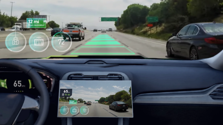
For example, Level 2 and Level 3 AI-assisted vehicles require the driver to remain in the loop during vehicle operation. Safe visualization inside the cockpit and the digital instrument cluster is key to ensuring the human driver is aware of how the system is perceiving and reacting to the surrounding environment. 

The confidence view is a rendering of the mind of the vehicle’s AI and how it sees the world. It shows exactly what the sensor suite and perception system are detecting in real time using a 3D surround model. By incorporating this view in the cabin interior, the vehicle can communicate to its occupants the accuracy and reliability of the autonomous driving system at every step of the journey.

The ability to support such in-vehicle graphics safely and securely is what makes Vulkan SC critical to the next-generation intelligent vehicle experience. Production Vulkan SC 1.0 drivers are included in DRIVE OS 6.0.4.0, which shipped August 29, 2022.

Vulkan SC on the NVIDIA Jetson embedded platform

NVIDIA Jetson is the world’s leading platform for autonomous machines and other embedded applications. It includes Jetson modules, which are small form-factor, high-performance computers, the NVIDIA JetPack SDK for accelerating software, and an ecosystem with sensors, SDKs, services, and products to speed development.

Applications for Jetson-based systems typically do not require formal safety certification. However, many embedded and autonomous systems can directly benefit from the deterministic, real-time GPU graphics and compute acceleration provided by Vulkan SC. With these capabilities, the Jetson platform can support a broader diversity of applications.

The NVIDIA Jetpack 5.0.2 SDK released on August 15 2022 includes conformant, production Vulkan SC 1.0 drivers for the Linux OS.

Ongoing NVIDIA commitment to the Vulkan SC API

NVIDIA will continue to invest in the evolution of the Vulkan SC open standard API at Khronos. We are committed to providing conformant, production drivers on platforms such as NVIDIA DRIVE and Jetson.

Later in 2022, NVIDIA will also ship support for Vulkan SC in NVIDIA Nsight developer tools. Vulkan SC streamlines the open, cross-platform Vulkan API for deterministic GPU graphics and compute, enabling advanced applications and use cases on safety-certified and real-time embedded platforms.

Now, NVIDIA provides industry-leading support for this groundbreaking open standard, enabling GPU acceleration in new classes of products. Download the latest NVIDIA DRIVE or NVIDIA Jetpack releases with Vulkan SC drivers today.

Categories
Misc

Top Manufacturing Sessions at GTC 2022

Discover the latest innovations in manufacturing and aerospace with GTC sessions from leaders at Siemens, Boeing, BMW, and more.

Discover the latest innovations in manufacturing and aerospace with GTC sessions from leaders at Siemens, Boeing, BMW, and more.

Categories
Misc

Concept Designer Ben Mauro Delivers Epic 3D Trailer ‘Huxley’ This Week ‘In the NVIDIA Studio’

The gripping sci-fi comic Huxley was brought to life in an action-packed 3D trailer full of excitement and intrigue this week In the NVIDIA Studio.

The post Concept Designer Ben Mauro Delivers Epic 3D Trailer ‘Huxley’ This Week ‘In the NVIDIA Studio’ appeared first on NVIDIA Blog.

Categories
Misc

Scaling Data Pipelines: AT&T Optimizes Speed, Cost, and Efficiency with GPUs

It is well-known that GPUs are the typical go-to solution for large machine learning (ML) applications, but what if GPUs were applied to earlier stages of the…
It is well-known that GPUs are the typical go-to solution for large machine learning (ML) applications, but what if GPUs were applied to earlier stages of the data-to-AI pipeline?

For example, it would be simpler if you did not have to switch out cluster configurations for each pipeline processing stage. You might still have some questions:

  • Would this be practical from a cost perspective?
  • Could you still meet SLAs on a data-processing time budget for some near-real-time processing?
  • How difficult is it to optimize these GPU clusters?
  • If you optimized the configuration for one stage, would the same work for other stages?

At AT&T, these questions arose when our data teams were working to manage cloud costs while balancing simplicity at scale. We also observed that many of our data engineers and scientist colleagues were not aware of GPUs being an effective and efficient infrastructure on which to run more mundane ETL and feature engineering stages.

It was also not clear what the relative performance could be of CPU compared to GPU configurations. Our goal at AT&T was to run a few typical configuration examples to understand the difference.

In this post, we share our data pipeline analysis in terms of speed, cost, and full pipeline simplicity. We also provide insights on design considerations and explain how we optimized the performance and price of our GPU cluster. The optimization came from using the RAPIDS accelerator for Apache Spark, an open-source library that enables GPU-accelerated ETL and feature engineering.

SPOILER ALERT: We were pleasantly surprised that, at least for the examples examined, the use of GPUs for each pipeline stage proved to be faster, cheaper, and simpler!

Use cases

Data-to-AI pipelines include multiple stages of batch processing:

  • Data preparation or federation
  • Transformation
  • Feature engineering
  • Data extraction

Batch processing involves processing a large volume of data containing trillions of records. Batch processing jobs are generally optimized for either cost or performance depending on the SLA for that use case.

A good example of a batch processing job optimized for cost is creating features from call records, which go on to be used to train an ML model. On the other hand, a real-time, inference use case to detect fraud is optimized for performance. GPUs are often overlooked and considered to be expensive for these batch-processing stages of AI/ML pipelines.

These batch processing jobs often involve large joins, aggregation, ranking, and transformation operations. As you can imagine, AT&T has many data and AI use cases that involve batch processing:

  • Network planning and optimization
  • Fraud
  • Sales and marketing
  • Tax

Depending on the use case, these pipelines can use NVIDIA GPUs and RAPIDS Accelerator for Apache Spark to optimize costs or improve performance. 

For this analysis, we look at a couple of data-to-AI pipelines. The first uses feature engineering of call records for a marketing use case, and the second use case carries out an ETL transformation of a complex tax dataset.

Speeding up feature engineering and transformation with GPUs

Efficiently scaling data-to-AI pipelines remains a need for data teams. High-cost pipelines are processing hundreds of terabytes to petabytes of data on a monthly, weekly, or even daily basis.

When examining efficiency, it is important to identify optimization opportunities across all ETL and feature engineering stages and then compare speed, cost, and pipeline simplicity.

For our data pipeline analysis, we compared three options:

To gauge how far we were from the optimum cost, we compared a bare-bone VM solution using AT&T’s open-sourced GS-lite solution that enables you to write SQL that then compiles to C++.

As mentioned earlier, after optimizing each solution, we discovered that the RAPIDS accelerator for Apache Spark running on a GPU cluster, had the best overall speed, cost, and design simplicity trade-off.

In the following sections, we discuss the chosen optimizations and design considerations for each.

Design considerations for optimizing the AI/ML pipeline solution

To compare the performance of the three potential solutions, we carried out two experiments, one for each of the selected use cases. For each, we optimized different parameters to gain insight into how speed, cost, and design are affected.

Example 1: Optimizing simple group by aggregations for the call-records use case

For the first feature engineering example, we chose to create features from call-record datasets containing close to three trillion records (rows) a month (Table 1). This data preprocessing use case is a fundamental building block in several sales and marketing AI pipelines, such as customer segmentation, predicting customer churn, and anticipating customer trends and sentiments. There were various data transformations in this use case, but many of them involved simple “group by” aggregations such as the following, for which we wanted to optimize the processing.

res=spark.sql("""
Select DataHour, dev_id, 
    sum(fromsubbytes) as fromsubbytes_total, 
    sum(tosubbytes) as tosubbytes_total, 
From df
Group By DataHour, dev_id
""")

Accessing insights from data and carrying out data analysis is still one of the biggest pain points for many enterprises. This is not because of lack of data, but because the amount of time spent on data preparation and analysis is still an impediment to data engineers and data scientists.

Here are some of the key infrastructure challenges in this preprocessing example:

  • Query execution on CPU cluster takes too long, leading to timeout issues.
  • The compute cost is expensive.
Days # of Rows Size (Bytes)
1 ~110 Billion >2 TB
7 ~800 Billion ~16 TB
30 ~3 Trillion ~70 TB
Table 1. Number of call records and data size

Also, this call-records use case had an extra dimension of experimentation in terms of compression types. The data was arriving from the network edge to the cloud with some form of compression that we could specify and evaluate tradeoffs for. We thus experimented with several compression schemes, including txt/gzip, Parquet/Z standard, and Parquet/Snappy.

The Z-standard compression had the smallest file size (about half in this case). As we show later, we found better speed/cost tradeoffs with Parquet/Snappy.

Next, we considered the type of cluster with regard to the number of cores per VM, number of VMs, the allocation of worker nodes, and whether to use a CPU or GPU.

  • For CPU clusters, we chose the lowest number of cores that could handle the workload, that is, the lowest number of VMs and workers to prevent an over-allocation of resources.
  • For GPUs, we used the RAPIDS Accelerator tuning guide [spark-rapids-tuning], which provides sizing recommendations with regard to concurrent tasks per executor, maxPartitionBytes, shuffle partitions, and concurrent GPU tasks.

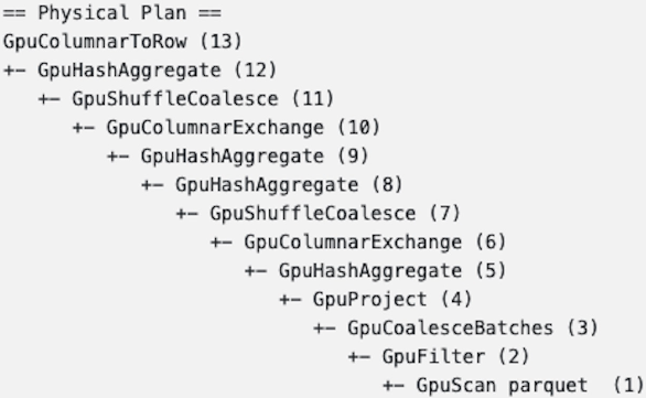
One goal after implementing the data processing on the GPU was to ensure that all key feature engineering steps remained on the GPU (Figure 1).

Spark GPU Physical plan showing information about execution of the query.
Figure 1. GPU physical processing plan

Example 2: Optimizing multiple ETL and feature creation stages for the tax dataset

The use case for Example 2 allowed us to compare many different transformations and processing stages for ETL, feature creation, and AI. Each stage had different record volume sizes (Figure 2).

Diagram shows the ETL/AI pipeline and transformations for each stage: filtering data, applying aggregations, AI fuzzy matches, many-to-many transformations, and generating reports.
Figure 2. ETL/AI flow and record volume sizes

This ETL pipeline with multiple stages is a common bottleneck in enterprises where data lives in silos. Most often massive data processing requires querying and joining data from two or more data sources using fuzzy logic. As you can see from Figure 2, even though we started only with 20 million rows of data, the data volume grew exponentially as we moved through the data processing stages.

As in Example 1, the design considerations were the number of cores per VM, number of VMs, and the allocation of worker nodes, when comparing CPUs and GPUs.

Results

After trying different core, worker, and cluster configurations for the use cases shown in examples 1 and 2, we collected the results. We ensured that any particular ETL job finished within the allocated time to keep up with the data input data rate. The best approach in both had the lowest cost and highest simplicity. 

Example 1 results

Figure 3 shows the cost/speed tradeoffs across a range of setups for simple group by aggregations in the call records use case. You can make several observations:

  • The lowest cost and simplest solution is using the GPU cluster with Snappy compression, being ~33% cheaper than the lowest-cost Photon solution and close to half the cost of the fastest Photon solution.
  • All standard Databricks clusters performed worse on both cost and execution time. Photon was the best CPU solution.

While not shown in Figure 3, the GS-lite solution was actually the cheapest, needing only two VMs.

Bar chart and line chart of execution time and cost for the RAPIDS Accelerator for Apache Spark, different CPU cluster VMs, and Databricks Photon.
Figure 3. Cost/execution and time tradeoffs for different Databricks cluster configurations

Example 2 results

Like Example 1, we tried several CPU and GPU cluster configurations for the five ETL and AI data processing stages with the Databricks 10.4 LTS ML runtime. Table 2 shows the resulting best configurations.

Configuration CPU GPU
Worker type Standard_D13_v2  56 GB memory, 8 cores, min workers 8, max workers 12 Standard_NC8as_T4_v3 56 GB memory, 1 GPU, min workers 2, max workers 16
Driver type Standard_D13_v2 56 GB memory, 8 cores Standard_NC8as_T4_v3 56 GB memory, 1 GPU
Table 2. Cloud VM instances for CPU and GPU

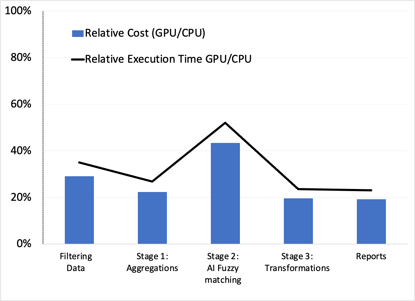
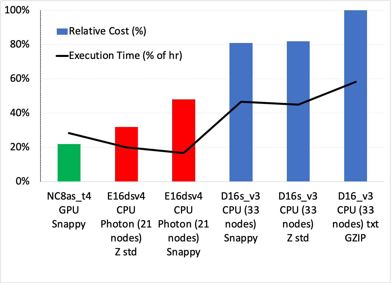
These configurations yielded the relative cost and execution time (speed) performances favoring GPUs (Figure 4).

Bar chart and Line chart showing relative cost and execution time of GPUs compared to CPUs.
Figure 4. Cost and execution-time tradeoffs

While not shown here, we confirmed that the next stages of the AI pipeline in Example 1, which used XGBoost modeling, also benefited from GPUs and RAPIDS Accelerator for Apache Spark. This confirms that GPUs could be the best end-to-end solution.

Conclusion

While not exhaustive of all AT&T’s data and AI pipelines, it appears that GPU-based pipelines were beneficial in all examples examined. In these cases, we were able to cut down the time for data preparation, model training, and optimization. This resulted in spending less money with a simpler design, as there was no configuration switching across stages.

We encourage you to experiment with your own data to AI pipelines, especially if you’re already using GPUs for AI/ML training. You may also find that GPUs are your “go-to,” simpler, faster, and cheaper solution!

Interested in learning more about these use cases and experiments, or getting tips on how to cut down your data processing time with the RAPIDS Accelerator for Apache Spark? Register for the free AT&T GTC session, How AT&T Supercharged their Data Science Efforts.

Categories
Misc

Top Telecommunications Sessions at GTC 2022

Join us for sessions from AT&T, Verizon, T-Mobile, Ericsson, and more to discover the latest innovations in telecom.

Join us for sessions from AT&T, Verizon, T-Mobile, Ericsson, and more to discover the latest innovations in telecom.

Categories
Misc

Improving Japanese Language ASR by Combining Convolutions with Attention Mechanisms

Automatic speech recognition (ASR) research generally focuses on high-resource languages such as English, which is supported by hundreds of thousands of hours…
Automatic speech recognition (ASR) research generally focuses on high-resource languages such as English, which is supported by hundreds of thousands of hours of speech. Recent literature has renewed focus on more complex languages, such as Japanese. Like other Asian languages, Japanese has a vast base character set (upwards of 3,000 unique characters are used in common vernacular), and poses unique challenges, such as multiple word order.

To learn more about the technology discussed in this post, watch the author’s INTERSPEECH 2022 presentation on September 20, Neural Transducers, Streaming ASR, and Novel ASR Models.

This post discusses recent work that improved both accuracy and speed for Japanese language ASR. First, we improved Conformer, a state-of-the-art ASR neural network architecture, to achieve a significant improvement in training and inferencing speed without accuracy loss. Second, we enhanced a pure and deep convolutional network with a multiple-head self attention mechanism for enriching the learning of global contextual representations of the input speech waves.

Deep sparse conformer for speech recognition

Conformer is a neural network architecture widely used in the ASR systems of numerous languages and has achieved high levels of accuracy. However, Conformer is relatively slow at both training and inferencing because it uses multi-head self-attention with a time/memory complexity of quadratic to the length of input audio waves. 

This prevents its efficient processing of long audio sequences since relatively high memory footprints are required during training and inferencing. These motivate the usage of sparse attention for efficient Conformer constructing. In addition, with sparse attention and relatively low memory cost, we are able to build a deeper network that can process long sequences fed with large-scale speech datasets.

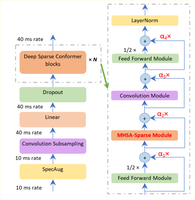
Diagram showing encoder model architecture for the deep sparse Conformer. A wave file is first sent to the spectrogram augmentation (SpecAug) module and then a convolutional subsampling network followed by a linear projection and a dropout function for preprocessing. Then, there are a stack of deep sparse Conformer building Macaron blocks in which two feed forward modules clamp a multi-head sparse self attention module and a convolution module.
Figure 1. Encoder model architecture for the deep sparse Conformer

As depicted in Figure 1, we improved the Conformer long-sequence representation ability in two directions: sparser and deeper. We used a ranking criteria to only select a small scale of dominant queries instead of the whole query set to save time for attention score computing.

A deep normalization strategy is used when performing residual connections to ensure the training of hundred-level Conformer blocks. This strategy involves discounting the parameters of the encoder and decoder parts with a function that is related respectively to the number of encoder layers and decoder layers.

In addition, this deep normalization strategy ensures a successful building of 10 to 100 layers so that the model is more expressive. In contrast, the deep sparse Conformer time and memory costs decrease at a rate of 10% to 20% when compared to the usual Conformer. 

Attention-enhanced Citrinet for speech recognition

Citrinet, proposed by NVIDIA researchers, is an end-to-end convolutional Connectionist Temporal Classification (CTC)-based ASR model. To capture local and global contextual information, Citrinet uses 1D time-channel separable convolutions combined with sub-word encoding and squeeze-and-excitation (SE), enabling the whole architecture to achieve state-of-the-art accuracies compared with transformer-based counterparts.

Applying Citrinet to Japanese ASR involves several challenges. Specifically, it is relatively slower at convergence and more difficult to train a model with a comparable accuracy than similar deep neural network models. Considering that there are as many as 235 convolutional layers that influence the convergence speed of Citrinet, we aim to reduce the CNN layers by introducing multi-head attentions in the convolution module in Citrinet blocks while keeping the SE and residual modules unchanged.

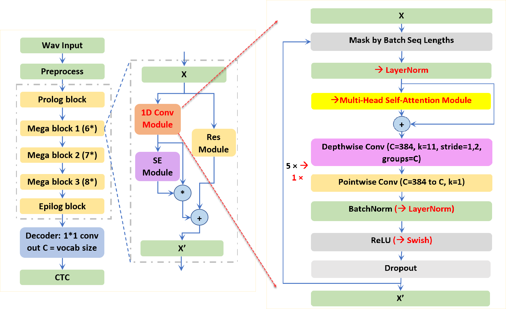
Diagram showing the Citrinet end-to-end architecture and major building block. 1D time-channel separable convolution and SE-attached Jasper Block, updated with multi-head self-attention module with layer normalization and reduced repeating number from 5 to 1.
Figure 2. The Citrinet end-to-end architecture and major building block

As shown in Figure 2, speeding up the training time involves reducing eight convolution layers in each attention-enhanced Citrinet block. In addition, considering that self-attention has time/memory complexities of quadratic to the length of input audio waves, we reduced the original 23 Jasper blocks to eight blocks with a significant model size reduction. This design ensures the attention-enhanced Citrinet reaches comparable inference time for long speech sequences with layers from the 20s to the 100s.

Preliminary experiments show that attention-based models converge at 100 to 200 epochs while 500 to 1,000 epochs are required for Citrinet’s convergence to the best error rates. Experiments on the Japanese CSJ-500-hour dataset show that the attention-Citrinet requires fewer layers of blocks and converges faster with lower character error rates than Citrinet with 80% training time and Conformer with 40% training time and 18.5% model size.

Summary

Generally, we propose two novel architectures to build end-to-end Japanese ASR models. In one direction, we improved the transformer-based Conformer training and inferencing speed and retained its accuracy. We successfully built sparser and deeper Conformer models. We also improved the CNN-based Citrinet convergence speed and accuracy by introducing a multi-head self-attention mechanism and pruning 80% of the CNN layers. These proposals are general and applicable to other Asian languages.

To learn more about Japanese language ASR models, see Deep Sparse Conformer for Speech Recognition and Attention Enhanced Citrinet for Speech Recognition, or watch the related INTERSPEECH 2022 session, Neural Transducers, Streaming ASR, and Novel ASR Models.

Categories
Misc

Changing CTC Rules to Reduce Memory Consumption in Training and Decoding

Loss functions for training automatic speech recognition (ASR) models are not set in stone. The older rules of loss functions are not necessarily optimal….
Loss functions for training automatic speech recognition (ASR) models are not set in stone. The older rules of loss functions are not necessarily optimal. Consider connectionist temporal classification (CTC) and see how changing some of its rules enables you to reduce GPU memory, which is required for training and inference of CTC-based models and more.

For more information about the technology behind this post, tune into the author’s presentation at INTERSPEECH 2022 on Monday, September 19, 14:30-16:30 (KST), Virtual Poster: Novel models and training methods for ASR II.

Overview of connectionist temporal classification

If you are going to train an ASR model, whether it’s a convolutional or recurrent neural network, a transformer, or a combination, you are most likely training it with the CTC loss. 

CTC is simple and convenient because it does not require per-frame information about “what sound is pronounced when” (so-called audio-text time alignment). In most cases, this knowledge is simply unavailable, as in a typical ASR dataset of audio with associated text with no time marks. 

True time alignment is not always trivial. Suppose that most of the recording is without speech with only one short phrase at the end. CTC loss does not tell the model when exactly to emit a prediction. Instead, it allows for every possible alignment and just regulates the form of these alignments.

Here’s how exactly CTC manages all possible ways to align audio against text. 

First, the target text is tokenized, that is, words are sliced into letters or word pieces. The number of the resulting units (whatever they are) should be less than the number of audio “timeframes”: segments of audio of length 0.01 to 0.08 seconds. 

If there are fewer timeframes than units, then the algorithm fails. In this case, you should make your timeframes shorter. Otherwise, only RNN Transducer can save you. If the timeframes are as many as the units, then there can be only one alignment (a one-in-a-million case). 

Most of the time, there are way more timeframes than units, so some of the frames are left without a unit. For such empty frames, CTC has a special unit. This unit tells you that the model has nothing to give you at this particular frame. This may be because there is no speech, or maybe the model is just too lazy to predict something meaningful here. The ability to predict nothing if the model doesn’t want to do that is provided by the most important rule of the CTC: the rule.

Other rules are related to unit continuation. Suppose that your unit is a vowel that lasts longer than one frame. On which of two frames should the model output the unit? CTC allows for the same unit emission on multiple consecutive frames. But then, the same consecutive units should be merged into one to convert the recognition results into a sequence of units that resembles text. 

Now, what if your tokenized text itself contains the same repeated units like “ll” or “pp”? If left unprocessed, these units are merged into one even if they shouldn’t be. For this special case, CTC has a rule that if the target text has repeated units, then such units must be separated by during inference. 

To sum up, in almost every frame, the model is allowed to emit the same unit from the previous frame, , or the next unit if it is different from the previous one. These rules are more sophisticated than the rule and they are not exactly necessary for CTC to work.

CTC implementation

Here’s how CTC loss can be represented. Like most loss functions in machine learning, it is usually represented as a dynamic algorithm that applies these rules to a training utterance or to the model’s softmax output. 

In training, loss values and gradients are computed from conditional probabilities of all possible alignments by the Baum–Welch algorithm, applied to the CTC rules. The CTC implementations often have hundreds to thousands of lines of code and can be hard to modify.

Fortunately, there is another way to implement CTC. The weighted finite-state transducers (WFST) approach, apart from other application areas, allows the model to represent a dynamic algorithm as a set of graphs and associated graph operations. This approach enables you to decouple the CTC rules by applying them to specific audio and text and by calculating loss and gradients.

CTC WFST applications

With WFST, you can easily take the CTC rules and use them with different criteria, like maximum mutual information (MMI). These models usually have a lower word error rate (WER) than CTC models. MMI incorporates prior language information into the training process. 

In contrast to CTC, MMI not only maximizes the probability of the most feasible path but also minimizes the probabilities of every other path. To do this, MMI has a so-called denominator graph, which can occupy a lot of  GPU memory during training. Fortunately, some CTC rules can be modified to reduce denominator memory consumption without compromising speech recognition accuracy.

Also, a WFST representation of CTC rules, or a so-called topology, can be used to allow for WFST decoding of CTC models. To do that, you convert an N-gram language model to a WFST graph and compose it with the topology graph. The resulting decoding graph can be passed to, for example, the Riva CUDA WFST Decoder

Decoding graphs can be large to the point that they may not fit in GPU memory. But with some CTC topology modifications, you can reduce decoding graph sizes for CTC.

CTC topologies

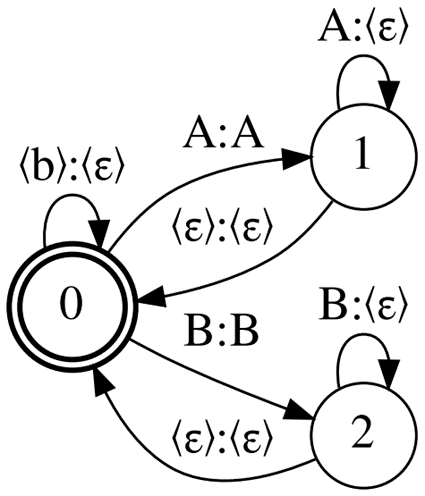
Figure 1 shows the CTC topology, Correct-CTC. This is a directed complete graph with self-loops, so for N units, including blank, there are N states and the square number of arcs. 

Correct-CTC is the most commonly used CTC representation. Look at the typical sizes that this topology produces. For the LibriSpeech 4-gram word language model and 256 units of the model vocabulary, the decoding graph size is ~16Gb. Cold-start MMI training on a 32Gb GPU with the model vocabulary size 2048 is possible only with batch size 1.

A fully-connected WFST with three nodes: 0 for <blank>, 1 for A, and 2 for B. Each node has a self-loop arc with the node’s unit as input and <epsilon> as output. Every node has arcs to all other nodes with arcs’ units according to the destination node.
Figure 1. Correct-CTC example for a three-unit vocabulary: , A, and B

Reduce the memory consumption induced by Correct-CTC by dropping some of the CTC rules. First, drop the mandatory separation of repeated units with . Without this rule, you end up with the topology called Compact-CTC ( Figure 2). It has 3N – 2 arcs for N units. 

A WFST with three nodes: 0 for <blank>, 1 for A, and 2 for B. Each node has a self-loop arc with the node’s unit as input and <epsilon> as output. The <blank> node has arcs to all other nodes with arcs’ units according to the destination node. Other nodes are connected to the <blank> node through (virtual) <epsilon>-arcs.
Figure 2. Compact-CTC example

Despite having pure epsilon (virtual) arcs, this topology can be used in training and decoding and does not negatively affect the recognition quality. If you’re wondering how this works, see CTC Variations Through New WFST Topologies or the NVIDIA NeMo implementation.

Decoding graph sizes with Compact-CTC are a quarter smaller than with Correct-CTC. It also requires 2x less GPU memory for MMI training.

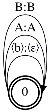
Now drop the same unit emission on multiple consecutive frames, leaving only the rule. This way, you end up with a topology with only one state and N arcs for N units. 

This is the smallest possible CTC topology, so we call it Minimal-CTC (Figure 3). It requires even less GPU memory for MMI training (4x less compared to Correct-CTC), but the accuracy of an MMI-trained model with the Minimal-CTC topology will degrade compared to the baseline. 

The smallest topology also produces the smallest decoding WFSTs with half the size of the baseline graph. Decoding graphs compiled with Minimal-CTC are incompatible with models built with Correct-CTC or Compact-CTC.

A WFST with a single node and three self-loop arcs for <blank>, A, and B.
Figure 3. Minimal-CTC example

Finally, l come back to Correct-CTC but this time leave mandatory separation of repeated units and drop unit continuation. The topology called Selfless-CTC was designed to remedy the shortcomings of Minimal-CTC. 

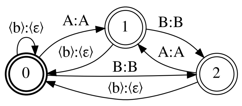
Figures 1 and 4 show that Correct-CTC and Selfless-CTC differ only in non- self-loops. These two topologies also give the same MMI model accuracy and an even better one if the model has a long context window. However, Selfless-CTC is also compatible with Minimal-CTC at decoding. You get the 2x graph size reduction from Minimal-CTC by the cost of only 0.2% higher WER.

A fully connected WFST with three nodes: 0 for <blank>, 1 for A, and 2 for B. The <blank> node has a self-loop arc with input <blank> and output <epsilon>. Every node has arcs to all other nodes with arcs’ units according to the destination node.
Figure 4. Selfless-CTC example; based on Correct-CTC

Conclusion

There are several tips for better performance:

  • Use Compact-CTC instead of Correct-CTC for decoding graph construction and MMI training.
  • For the best decoding graph size reduction, train your models with Selfless-CTC and decode with Minimal-CTC.
  • Loss functions are not set in stone:  Experiment with your own WFST representations of existing loss functions and create new ones. It’s fun!

For more information, see CTC Variations Through New WFST Topologies or view the INTERSPEECH session.

Other useful resources: