Categories
Misc

Improving Diffusion Models as an Alternative To GANs, Part 2

Researchers at NVIDIA have developed methods to improve and accelerate sampling from diffusion models, a novel and powerful class of generative models.

This is part of a series on how researchers at NVIDIA have developed methods to improve and accelerate sampling from diffusion models, a novel and powerful class of generative models. Part 1 introduced diffusion models as a powerful class for deep generative models and examined their trade-offs in addressing the generative learning trilemma.

While diffusion models satisfy both the first and second requirements of the generative learning trilemma, namely high sample quality and diversity, they lack the sampling speed of traditional GANs. In this post, we review three recent techniques developed at NVIDIA for overcoming the slow sampling challenge in diffusion models. 

Latent space diffusion models

One of the main reasons why sampling from diffusion models is slow is that mapping from a simple Gaussian noise distribution to a challenging multimodal data distribution is complex. Recently, NVIDIA introduced the Latent Score-based Generative Model (LSGM), a new framework that trains diffusion models in a latent space rather than the data space directly. 

In LSGM, we leverage a variational autoencoder (VAE) framework to map the input data to a latent space and apply the diffusion model there. The diffusion model is then tasked with modeling the distribution over the latent embeddings of the data set, which is intrinsically simpler than the data distribution.

Novel data synthesis is achieved by first generating embeddings through drawing from a simple base distribution followed by iterative denoising, and then transforming this embedding using a decoder to data space (Figure 1).

The data and latent spaces are mapped to each other using autoencoders. A diffusion model is formed on the latent encoding of the data.
Figure 1. Latent score-based generative model

Figure 1 shows that in the latent score-based generative model (LSGM),

  • Data x is mapped to latent space through an encoder q(z_0|x).
  • A diffusion process is applied in the latent space (z_0 rightarrow z_1).
  • Synthesis starts from the base distribution p(z_1).
  • It generates samples z_0 in latent space through denoising (z_0 leftarrow z_1).
  • The samples are mapped from latent to data space using a decoder p(x|z_0).
  • The model is trained end-to-end.

LSGM has several key advantages: synthesis speed, expressivity, and tailored encoders and decoders.

Synthesis speed

By pretraining the VAE with a Gaussian prior first, you can bring the latent encodings of the data distribution close to the Gaussian prior distribution, which is also the diffusion model’s base distribution. The diffusion model only has to model the remaining mismatch, resulting in a much less complex model from which sampling becomes easier and faster.

The latent space can be tailored accordingly. For example, we can use hierarchical latent variables and apply the diffusion model only over a subset of them or at a small resolution, further improving synthesis speed.

Expressivity

Training a regular diffusion model can be considered as training a neural ODE directly on the data. However, previous works found that augmenting neural ODEs, as well as other types of generative models, with latent variables often improves their expressivity.

We expect similar expressivity gains from combining diffusion models with a latent variable framework.

Tailored encoders and decoders

As you use the diffusion model in latent space, you can use carefully designed encoders and decoders mapping between latent and data space, further improving synthesis quality. The LSGM method can therefore be naturally applied to noncontinuous data.

Results

In principle, LSGM can easily model data such as text, graphs, and similar discrete or categorical data types by using encoder and decoder networks that transform this data into continuous latent representations and back.

Regular diffusion models that operate on the data directly could not easily model such data types. The standard diffusion framework is only well defined for continuous data, which can be gradually perturbed and generated in a meaningful manner.

Experimentally, LSGM achieves state-of-the-art Fréchet inception distance (FID), a standard metric to quantify visual image quality, on CIFAR-10 and CelebA-HQ-256, two widely used image generation benchmark data sets. On those data sets, it outperforms prior generative models, including GANs.

On CelebA-HQ-256, LSGM achieves a synthesis speed that is faster than previous diffusion models by two orders of magnitude. LSGM requires only 23 neural network calls when modeling the CelebA-HQ-256 data, compared to previous diffusion models trained on the data space that often rely on hundreds or thousands of network calls.

Video 1. Sequence generated by randomly traversing the latent space of LSGM.

Critically damped Langevin diffusion

A crucial ingredient in diffusion models is the fixed forward diffusion process to gradually perturb the data. Together with the data itself, it uniquely determines the difficulty of learning the denoising model. Hence, can we design a forward diffusion that is particularly easy to denoise and therefore leads to faster and higher-quality synthesis?

Diffusion processes like the ones employed in diffusion models are well studied in areas such as statistics and physics, where they are important in various sampling applications. Taking inspiration from these fields, we recently proposed critically damped Langevin diffusion (CLD)

In CLD, the data that must be perturbed are coupled to auxiliary variables that can be considered velocities, similar to velocities in physics in that they essentially describe how fast the data moves towards the diffusion model’s base distribution.

Like a ball that is dropped on top of a hill and quickly rolls into a valley on a relatively direct path accumulating a certain velocity, this physics-inspired technique helps the data to diffuse quickly and smoothly. The forward diffusion SDE that describes CLD is as follows:

large binom{d bf{x}_t}{d bf{v}_t} = underbrace{ binom{M^{-1} bf{v}_t}{-bf{x}_t} beta dt}_{Hamiltonian~component=: it{H}} + underbrace{ binom{ bf{0}_d}{-Gamma M^{-1}v_t} beta dt + binom{0}{sqrt{2 Gamma beta}} d bf{w}_t}_{Ornstein-Uhlenbeck~process=: it{O}}

Here, x_t denotes the data and v_t the velocities. M, Gamma, and beta are parameters that determine the diffusion as well as the coupling between velocities and data. Furthermore, dw_t is a Gaussian white noise process, responsible for noise injection, as seen in the formula.

CLD can be interpreted as a combination of two different terms. First is an Ornstein-Uhlenback process, the particular kind of noise injection process used here, which acts on the velocity variables v_t.

Second, the data and velocities are coupled to each other as in Hamiltonian dynamics, such that the noise injected into the velocities also affects the data x_t. Hamiltonian dynamics provides a fundamental description of the mechanics of physical systems, like the ball rolling down a hill from the example mentioned earlier.

Figure 2 shows how data and velocity diffuse in CLD for a simple one-dimensional toy problem:
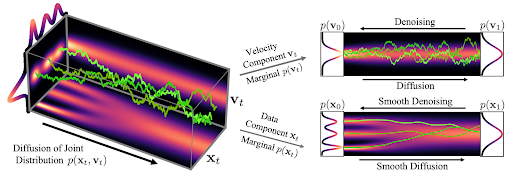
Visualization of critically-damped Langevin diffusion run in the joint data-velocity space using 1D toy distributions.
Figure 2. In critically-damped Langevin diffusion, the data xt is augmented with a velocity vt. A diffusion coupling xt and vt is run in the joint data-velocity space (probabilities in red). Noise is injected only into vt. This leads to smooth diffusion trajectories (green) for the data xt.

At the beginning of the diffusion, we draw a random velocity from a simple Gaussian distribution and the full diffusion then takes place in the joint data-velocity space. When looking at the evolution of the data (lower right in the figure), the model diffuses in a significantly smoother manner than for previous diffusions.

Intuitively, this should also make it easier to denoise and invert the process for generation. We obtain this behavior only for a particular choice of the diffusion parameters M and Gamma, specifically for Gamma^2 = 4M. This configuration is known as critical damping in physics and corresponds to a special case of a broader class of stochastic dynamical systems known as Langevin dynamics—hence the name critically damped Langevin diffusion.

We can also visualize how images evolve in the high-dimensional joint data-velocity space, both during forward diffusion and generation:
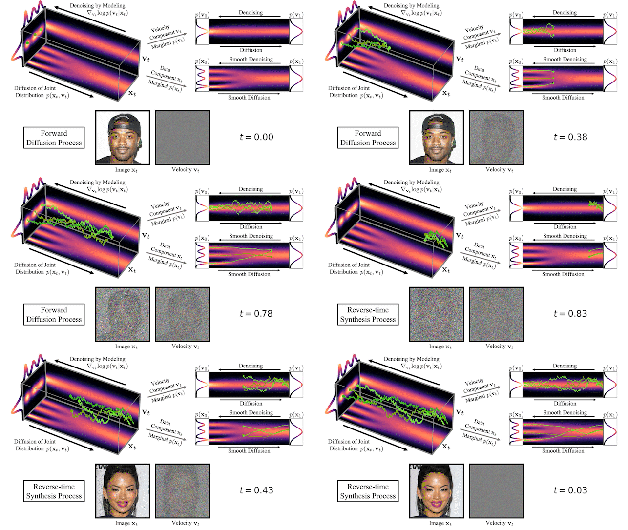
Animation of critically-damped Langevin diffusion’s forward diffusion and reverse-time synthesis processes.
Figure 3. CLD’s forward diffusion and the reverse-time synthesis processes

At the top of Figure 3, we visualize how a one-dimensional data distribution together with the velocity diffuses in the joint data-velocity space and how generation proceeds in the reverse direction. We sample three different diffusion trajectories and also show the projections into data and velocity space on the right. At the bottom, we visualize a corresponding diffusion and synthesis process for image generation. We see that the velocities “encode” the data at intermediate times t.

Using CLD when training generative diffusion models leads to two key advantages:

  • Simpler score function and training objective
  • Accelerated sampling with tailored SDE solvers

Simpler score function and training objective

In regular diffusion models, the neural network is tasked with learning the score function nabla_{x} log ~p_t (x) of the diffused data distribution. In CLD-based models, in contrast, we are tasked with learning nabla_{v} log ~p_t (v|x_t), the conditional score function of the velocity given the data. This is a consequence of injecting noise only into the velocity variables.

However, as the velocity always follows a smoother distribution than the data itself, this is an easier learning problem. The neural networks used in CLD-based diffusion models can be simpler, while still achieving high generative performance. Related to that, we can also formulate an improved and more stable training objective tailored to CLD-based diffusion models.

Accelerated sampling with tailored SDE solvers

To integrate CLD’s reverse-time synthesis SDE, you can derive tailored SDE solvers for more efficient denoising of the smoother forward diffusion arising in CLD. This results in accelerated synthesis.

Experimentally, for the widely used CIFAR-10 image modeling benchmark, CLD outperforms previous diffusion models in synthesis quality for similar neural network architectures and sampling compute budgets. Furthermore, CLD’s tailored SDE solver for the generative SDE significantly outperforms solvers such as Euler–Maruyama, a popular method to solve the SDEs arising in diffusion models, in generation speed. For more information, see Score-Based Generative Modeling with Critically-Damped Langevin Diffusion.
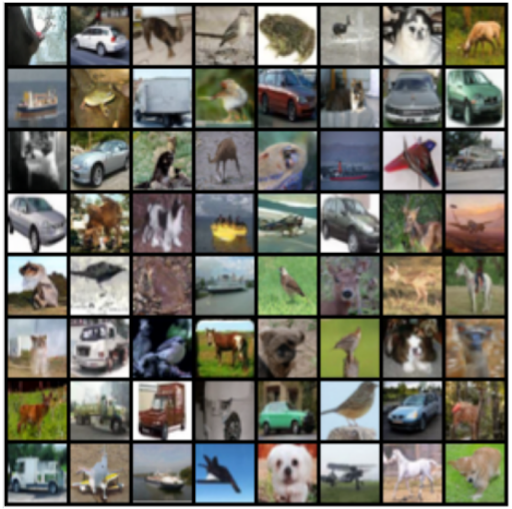
CIFAR-10 images generated by a diffusion model based on critically-damped Langevin diffusion.
Figure 4. Synthesized CIFAR-10 images generated by a diffusion model based on critically damped Langevin diffusion.

We’ve shown that you can improve diffusion models by merely designing their fixed forward diffusion process in a careful manner.

Denoising diffusion GANs

So far, we’ve discussed how to accelerate sampling from diffusion models by moving the training data to a smooth latent space as in LSGM or by augmenting the data with auxiliary velocity variables and designing an improved forward diffusion process as in CLD-based diffusion models.

However, one of the most intuitive ways to accelerate sampling from diffusion models is to directly reduce the number of denoising steps in the reverse process. In this part, we go back to discrete-time diffusion models, trained in the data space and analyze how the denoising process behaves as you reduce the number of denoising steps and perform large steps. ​

In a recent study, we observed that diffusion models commonly assume that the learned denoising distributions p_{ theta} (x_{t-1}|x_t) in the reverse synthesis process can be approximated by Gaussian distributions. However, it is known that the Gaussian assumption holds only in the infinitesimal limit of many small denoising steps, which ultimately leads to the slow synthesis of diffusion models. 

When the reverse generative process uses larger step sizes (has fewer denoising steps), we need a non-Gaussian, multimodal distribution for modeling the denoising distribution p_{ theta} (x_{t-1}|x_t).

Intuitively, in image synthesis, the multimodal distribution arises from the fact that multiple plausible and clean images may correspond to the same noisy image. Because of this multimodality, simply reducing the number of denoising steps, while keeping the Gaussian assumption in the denoising distributions, hurts generation quality.
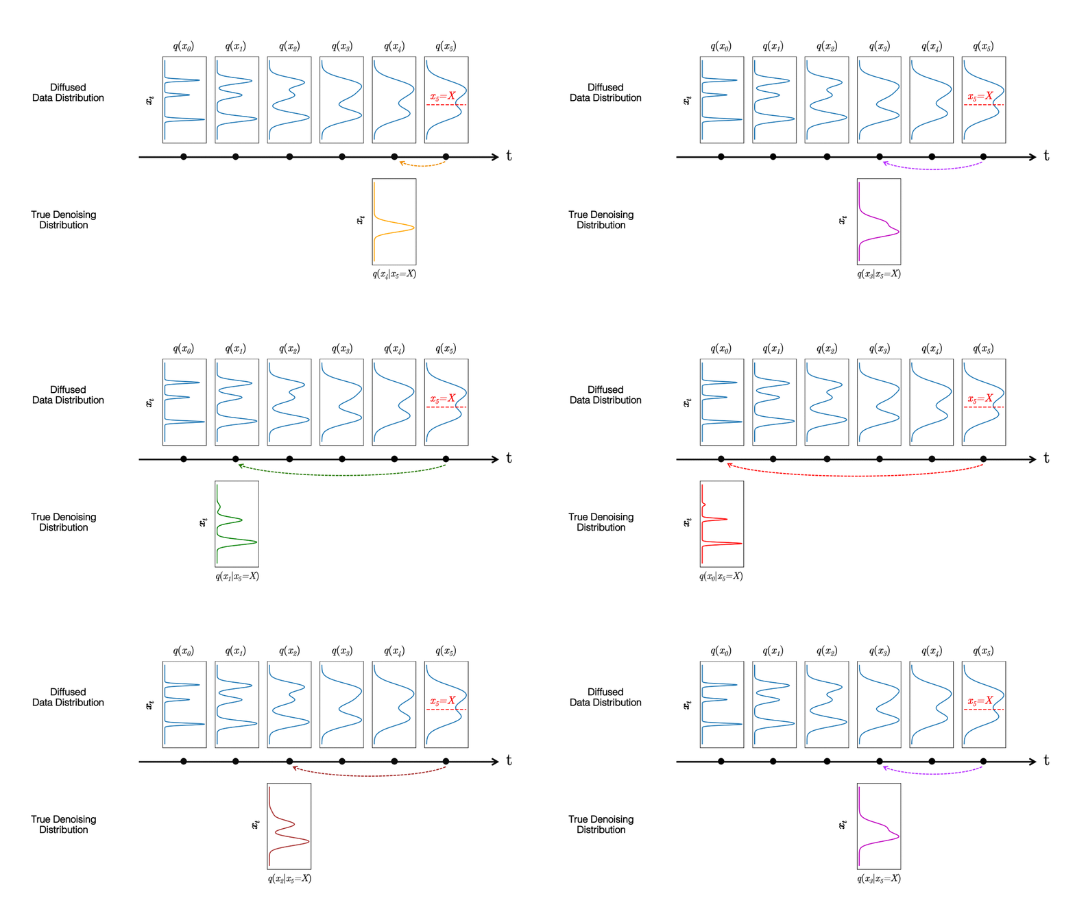
Visualization of diffused 1D data distributions in diffusion models and of the true denoising distributions for different step sizes during denoising.
Figure 5. (top) Evolution of a 1D data distribution q(x0) according to the forward diffusion process. (bottom) Visualizations of the true denoising distribution when conditioning on a fixed x5 with varying step sizes shown in different colors.

In Figure 5, the true denoising distribution for a small step size (shown in yellow) is close to a Gaussian distribution. However, it becomes more complex and multimodal as the step size increases.

Inspired by the preceding observation, we propose to parametrize the denoising distribution with an expressive multimodal distribution to enable denoising with large steps. In particular, we introduce a novel generative model, Denoising Diffusion GAN, in which the denoising distributions are modeled with conditional GANs (Figure 6).
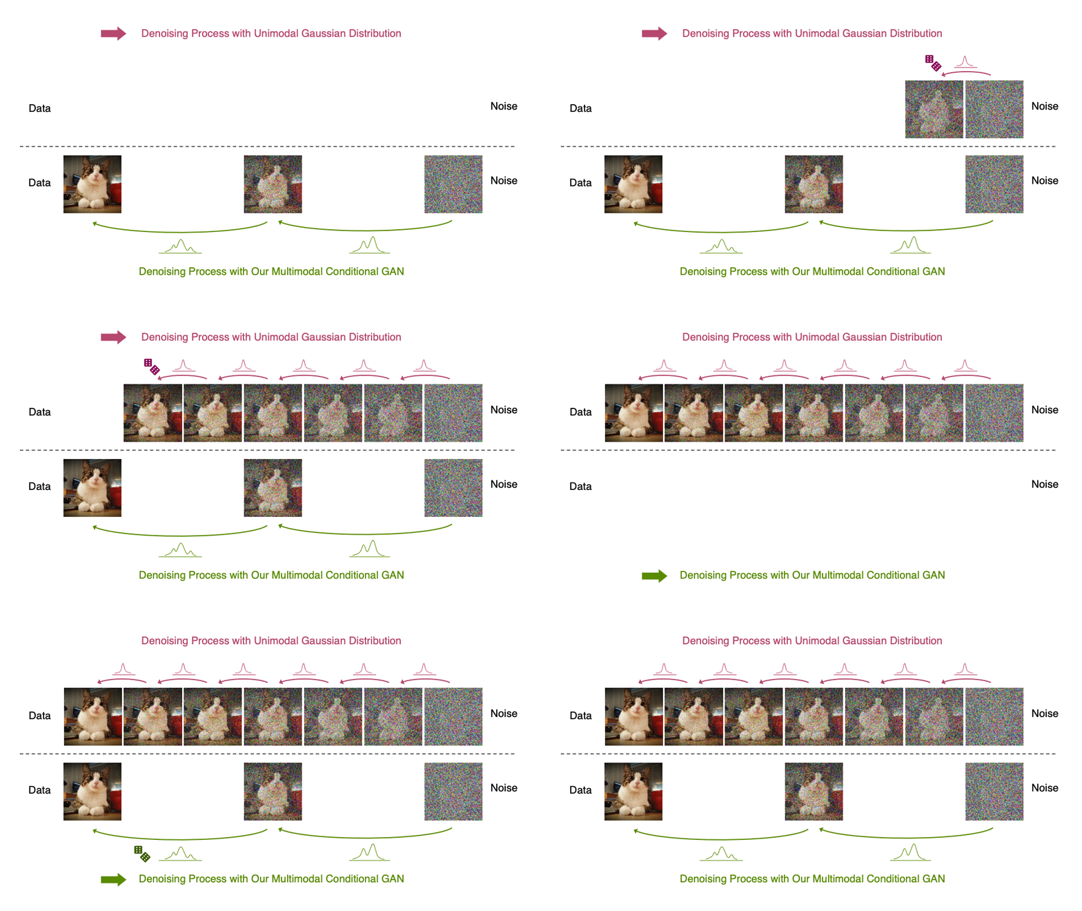
Visualization of the generative denoising process in diffusion models with Gaussian denoising distributions and with Denoising Diffusion GAN.
Figure 6. Denoising diffusion process

Generative denoising diffusion models typically assume that the denoising distribution can be modeled by a Gaussian distribution. This assumption holds only for small denoising steps, which in practice translates to thousands of denoising steps in the synthesis process.

In our Denoising Diffusion GANs, we represent the denoising model using multimodal and complex conditional GANs, enabling us to efficiently generate data in as few as two steps.

Denoising Diffusion GANs are trained using an adversarial training setup (Figure 7). Given a training image x_0, we use the forward Gaussian diffusion process to sample from both x_{t-1} and x_t, the diffused samples at two successive steps.

Given x_t, our conditional denoising GAN first stochastically generates x'_0 and then uses the tractable posterior distribution q(x'_{t-1}|x_t, x'_0) to generate x'_{t-1} by adding back noise. A discriminator is trained to distinguish between the real (x_{t-1}, x_t) and the generated (x'_{t-1}, x_t) pairs and provides feedback to learn the conditional denoising GAN.

After training, we generate novel instances by sampling from noise and iteratively denoising it in few steps using our Denoising Diffusion GAN generator.

Schematic visualization of the training pipeline of Denoising Diffusion GAN.
Figure 7. Training process of Denoising Diffusion GAN

We train a conditional GAN generator to denoise inputs x_t using an adversarial loss for different steps in the diffusion process.

Advantages over traditional GANs

Why not just train a GAN that can generate samples in one shot using a traditional setup, in contrast to our model that iteratively generates samples by denoising? Our model has several advantages over traditional GANs.

GANs are known to suffer from training instabilities and mode collapse. Some possible reasons include the difficulty of directly generating samples from a complex distribution in one shot, as well as overfitting problems when the discriminator only looks at clean samples. 

In contrast, our model breaks the generation process into several conditional denoising diffusion steps in which each step is relatively simple to model, due to the strong conditioning on x_t. The diffusion process smoothens the data distribution, making the discriminator less likely to overfit.

We observe that our model exhibits better training stability and mode coverage. In image generation, we observe that our model achieves sample quality and mode coverage competitive with diffusion models while requiring only as few as two denoising steps. It achieves up to 2,000x speed-up in sampling compared to regular diffusion models. We also find that our model significantly outperforms state-of-the-art traditional GANs in sample diversity, while being competitive in sample fidelity.
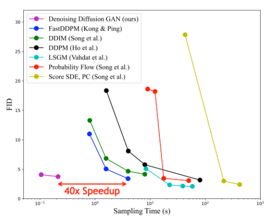
Plot of sample quality vs. sampling time for different denoising diffusion-based generative models.
Figure 8. Sample quality vs. sampling time for different diffusion-based generative models

Figure 8 shows sample quality (as measured by Fréchet inception distance; lower is better) compared to sampling time for different diffusion-based generative models for the CIFAR-10 image modeling benchmark. Denoising Diffusion GANs achieve a speedup of several orders of magnitude compared to other diffusion models while maintaining similar synthesis quality.

Conclusion

Diffusion models are a promising class of deep generative models due to their combination of high-quality synthesis and strong diversity and mode coverage. This is in contrast to methods such as regular GANs, which are popular but often suffer from limited sample diversity. The main drawback of diffusion models is their slow synthesis speed. 

In this post, we presented three recent techniques developed at NVIDIA that successfully address this challenge. Interestingly, they each approach the problem from different perspectives, analyzing the different components of diffusion models:

  • Latent space diffusion models essentially simplify the data itself, by first embedding it into a smooth latent space, where a more efficient diffusion model can be trained.
  • Critically damped Langevin diffusion is an improved forward diffusion process that is particularly well suited for easier and faster denoising and generation.
  • Denoising diffusion GANs directly learn a significantly accelerated reverse denoising process through expressive multimodal denoising distributions.

We believe that diffusion models are uniquely well-suited for overcoming the generative learning trilemma, in particular when using techniques like the ones highlighted in this post. These techniques can also be combined, in principle. 

In fact, diffusion models have already led to significant progress in deep generative learning. We anticipate that they will likely find practical use in areas such as image and video processing, 3D content generation and digital artistry, and speech and language modeling. They will also find use in fields such as drug discovery and material design, as well as various other important applications. We think that diffusion-based approaches have the potential to power the next generation of leading generative models.

Last but not least, we are part of the organizing committee for a tutorial on diffusion models, their foundations, and applications, held in conjunction with the Computer Vision and Pattern Recognition (CVPR) conference, on June 19, 2022, in New Orleans, Louisiana, USA. If you are interested in this topic, we invite you to see our Denoising Diffusion-based Generative Modeling: Foundations and Applications tutorial. 

To learn more about the research that NVIDIA is advancing, see NVIDIA Research.

For more information about diffusion models, see the following resources:

Categories
Misc

keras model.predict on a single image

I trained a model on MNIST, but I get an error when trying to use model.predict on a single image. Apparently keras model.predict can only take in batches of images. Why? Is there any way around this?

submitted by /u/berimbolo21
[visit reddit] [comments]

Categories
Misc

In the NVIDIA Studio: April Driver Launches Alongside New NVIDIA Studio Laptops and Featured 3D Artist

This week In the NVIDIA Studio, we’re launching the April NVIDIA Studio Driver with optimizations for the most popular 3D apps, including Unreal Engine 5, Cinema4D and Chaos Vantage. The driver also supports new NVIDIA Omniverse Connectors from Blender and Redshift.

The post In the NVIDIA Studio: April Driver Launches Alongside New NVIDIA Studio Laptops and Featured 3D Artist appeared first on NVIDIA Blog.

Categories
Misc

Accelerating Cloud-Ready Infrastructure and Kubernetes with Red Hat OpenShift and the NVIDIA BlueField DPU

An animated visualization of Red Hat Openshift running on the NVIDIA BlueField DPUTake a deep dive into the integrated cloud-ready infrastructure solution from Red Hat and NVIDIA An animated visualization of Red Hat Openshift running on the NVIDIA BlueField DPU
The IT world is moving to cloud, and cloud is built on containers managed with Kubernetes. We believe the next logical step is to accelerate this infrastructure with data processing units (DPUs) for greater performance, efficiency, and security.

Red Hat and NVIDIA are building an integrated cloud-ready infrastructure solution with the management and automation of Red Hat OpenShift combined with the acceleration, workload isolation, and security capabilities of NVIDIA BlueField DPUs.

Benefits of Red Hat OpenShift

Many popular cloud infrastructure projects use containers managed by Kubernetes. However, implementing Kubernetes can be a heavy lift, especially for organizations that cannot devote dedicated staff to becoming Kubernetes experts. 

Red Hat OpenShift provides a powerful set of capabilities for managing Kubernetes containers as well as application deployment, updates, and lifecycle management. OpenShift includes automation and security tools, as well as a supported open-source model to make cloud infrastructure more affordable, reliable, and scalable.

According to a 2021 Red Hat survey, Kubernetes is used for over 85% of container orchestration projects, and Red Hat OpenShift is the most popular choice for hybrid and multicloud Kubernetes deployments. OpenShift is the industry’s leading enterprise Kubernetes platform, used by more than 50% of commercial banks, telecommunications companies, and airlines on the Fortune 500.

It is clear that most enterprises want a supported Kubernetes model, and Red Hat OpenShift is one of the most popular choices.

How a DPU works

A DPU offloads, accelerates, and isolates infrastructure workloads from the server’s CPU. For example, the BlueField DPU can offload networking, network virtualization, data encryption, and time synchronization tasks from the CPU and run them on purpose-built silicon.

Other infrastructure software, such as remote management, firewall agents, network control plane, and storage virtualization, can run on BlueField’s Arm processor cores. Doing so frees up the server’s CPU cores that can instead run applications and tenant workloads.

This functionality also isolates infrastructure and security workloads in a separate domain. The result is a set of servers that run more applications with faster networking, increasing the efficiency and security of the data center. 

In a typical cloud infrastructure, the network traffic traverses both physical servers and containers running on these servers. This requires a packet switching solution within each server, and to gain maximum efficiency, the application containers need a way to talk to the accelerated networking offloads of the DPU.

The traditional way is to go through Kubernetes and Open Virtual Network (OVN) to access the Open Virtual Switch (Open vSwitch or OVS). OVN provides network abstraction and the default deployment strategy is to run both OVN and OVS on the host server’s CPU.

However, this method consumes a significant number of CPU cores as the network speeds increase beyond 10 Gbps. A solution is needed for Kubernetes to run the OVN and OVS functionality on the DPU so that all the packet switching, header rewrites, encapsulation/decapsulation, and packet filtering can be done on networking hardware instead of in software on the CPU. 

Increasing networking integration between Red Hat and NVIDIA

Red Hat and NVIDIA have collaborated to integrate the management power of OpenShift with the acceleration capabilities of the DPU.

The first stage of integration started in 2018 with Red Hat Enterprise Linux offloading network traffic to the NVIDIA ConnectX SmartNIC. The networking data plane–using OVS or DPDK–was running on the SmartNIC ASIC but the networking control plane was still running entirely in software on the X86 CPU.

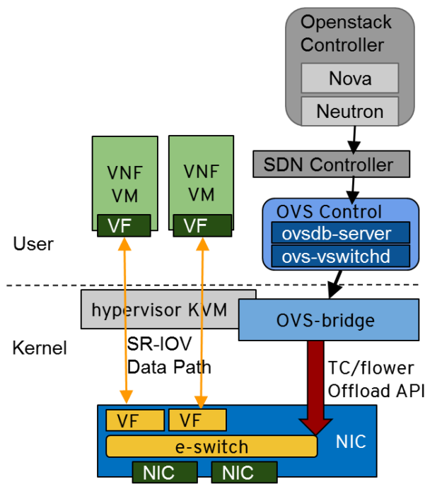
This is a diagram of the OpenStack software-defined networking (SDN) components running in Red Hat Enterprise Linux and interacting via Open vSwitch (OVS) with the eSwitch in the NVIDIA ConnectX SmartNIC. This integration allows the eSwitch hardware to offload and accelerate the SDN data plane packet switching for virtual machines running in user space.
Figure 1. OpenStack SDN controller, running on Red Hat Enterprise Linux, offloads the networking data plane to the NVIDIA ConnectX SmartNIC through OVS while the control plane runs on the X86 CPU.

In 2021, the companies took the next step and deployed Red Hat OpenShift with the NVIDIA BlueField DPU and ran performance benchmark tests. At NVIDIA GTC 2021, we demonstrated the advantages of shifting networking to the DPU and published a post, Optimizing server utilization in data centers by offloading network functions to NVIDIA BlueField-2 DPUs.

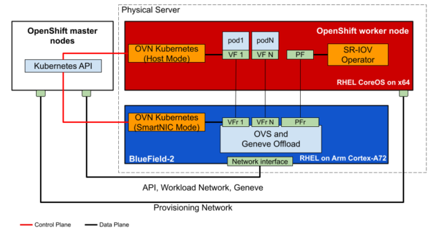
In this solution, the networking data plane with overlay offload (OVS and Geneve Offload) and the networking control plane (in the OVN Kubernetes pod) were running on the DPU with Red Hat Enterprise Linux. The major OpenShift components, including Red Hat Enterprise Linux CoreOS remained on the x86 CPU.

This diagram shows Red Hat OpenShift with Kubernetes running on the x86 CPU and offloading both the open virtual networking (OVN) data plane and control plane to the BlueField-2 DPU. Red Hat Enterprise Linux CoreOS is running only on the x86 CPU as the DPU runs Red Hat Enterprise Linux. The tenant containers/pods on the x86 host offload their networking virtual functions to the DPU.
Figure 2. Red Hat OpenShift, running on Red Hat Enterprise Linux CoreOS, offloads both the networking data plane and control plane to the BlueField-2 DPU, via OVN and OVS. The DPU is running Red Hat Enterprise Linux on its Arm cores.

In the deployment scenario in Figure 2, the BlueField-2 does the heavy lifting in the following areas: 

  • Geneve (virtual overlay network) encapsulation/decapsulation 
  • IPsec encapsulation/decapsulation 
  • Encryption/decryption routing
  • Network address translation (NAT)

The host CPU and container see only simple unencapsulated, unencrypted packets and the CPU does not need to perform any of these tasks because they are offloaded to the DPU. This level of offload reduced CPU utilization by 70%, freeing up substantial CPU power on each server to run additional business/tenant workloads. 

Running OpenShift on the DPU

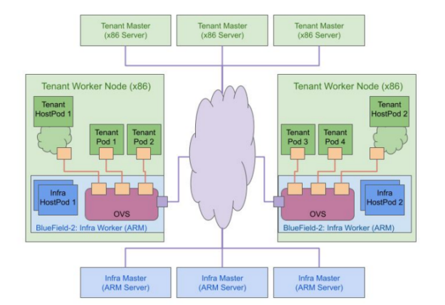
As presented at GTC 2022, Red Hat and NVIDIA have taken the next step, moving OpenShift, including Red Hat Enterprise Linux CoreOS, to run on the Arm cores of the BlueField DPU for the Red Hat OpenShift two cluster design that includes separate tenant and infrastructure clusters.

Red Hat Enterprise Linux CoreOS is the supported operating system for the OpenShift control plane, or master and worker nodes. This is the portion of OpenShift that performs scheduling, maintenance, upgrades, and cluster automation. It includes container management tools and security hardening to make it more resistant to hackers, and it now runs on both the host x86 CPU and on the DPU Arm cores.

BlueField DPUs running OpenShift OVS and OVN containers and Red Hat Enterprise Linux CoreOS on the various host servers form an infrastructure worker cluster. Meanwhile, OpenShift running on the x86 CPUs manages the tenant pods and clusters.

Offloading the OpenShift infrastructure cluster software to run on the BlueField Arm cores instead of on the host x86 cores provides additional x86 CPU savings, higher performance, and stronger security isolation.

Diagram shows that Red Hat OpenShift runs on both the host x86 CPUs and on the BlueField Arm cores. The X86 CPUs form an OpenShift tenant cluster while the DPUs on each server form an OpenShift infrastructure cluster.
Figure 3. Starting with Red Hat OpenShift 4.10, you can run OpenShift on both the x86 CPUs to manage the tenants and on the BlueField DPU Arm cores to manage the cluster infrastructure.

The cloud-native, software-defined networking is a good example of a BlueField DPU use case where OVN and OVS are running on and offloaded by the BlueField DPU in an OpenShift environment. Many other infrastructure services, such as network encryption, firewall agents, virtual routers, telemetry agents, and so on, can also be run on the DPU for an even greater benefit.

Significant cost savings benefits from OpenShift Offload on DPU 

To understand the impact of the DPU offloads on reducing the data center costs, NVIDIA and Red Hat put together a TCO model for a mid-sized data center with 51K servers. We considered this data center to be supporting 1M applications, each application needing 10K packets per second (PPS) of switching performance.

We considered two server deployment scenarios: with and without a DPU:

  • The server with no DPU running the virtual switching entirely in software achieved only 350k PPS.
  • The server with a DPU that offloads OVN and OVS to the DPU achieved 54x times higher performance of 18.7 million PPS per server.

Offloading virtual switching to the DPU also saved eight CPU cores per server. Based on this testing, the TCO model yielded amazing savings of $68.5M of CapEx. These savings are recognized by requiring 10K fewer DPU-enhanced servers due to much higher networking performance and CPU core savings per server.

We see power savings due to the smaller server footprint, which ultimately results in a better TCO model with the DPU-based servers. These TCO savings will get even better as we offload additional functions such as load balancers, firewalls, encryption, web servers, and so on to the DPUs, ultimately achieving amazing efficiency for cloud-ready data centers.

Solution roadmap and deploying OpenShift on BlueField 

The two-cluster OpenShift architecture running OpenShift on BlueField is now available as a developer preview or early trial in OpenShift 4.10, and is expected to become generally available in 2022.

But the NVIDIA and Red Hat teams aren’t stopping here. We are planning to test the offloading of network traffic encryption/decryption as that is a CPU-intensive task.

  • BlueField-2 DPU can offload IPsec encryption/decryption at up to 100 Gbps and TLS encryption/decryption at up to 200 Gbps.
  • BlueField-3 is expected to support IPSec, TLS and MACsec at even higher speeds.

Implementation of line-rate encryption offload from OpenShift to the DPU will improve data security for tenants and help you move closer to a zero-trust security stance.

Other potential integrations with the DPU include more sophisticated software-defined networking offloads, running a firewall agent on BlueField, precision time synchronization, video streaming with packet pacing, and using the DPU to collect telemetry data.

BlueField-2 DPUs are available now from NVIDIA and the BlueField-3 DPU will start sampling later in 2022. In addition, BlueField DPUs will soon be available for testing in the NVIDIA LaunchPad cloud service. 

If you would like to test or develop on Red Hat OpenShift running with the NVIDIA BlueField DPU, please indicate your interest

Summary

If your organization seeks to embrace cloud-native computing in data centers, the combination of NVIDIA BlueField DPUs, Red Hat Enterprise Linux, and Red Hat OpenShift provides an efficient and innovative open, hybrid-cloud platform with new security features. This powerful platform delivers hardware acceleration capabilities to run critical software-defined networking, storage, and security functions.

Now more server resources can be allocated to run cloud-native workloads, as well as traditional business applications.

For more information, see the following resources:  

Categories
Misc

9 Best Artificial Intelligence books for beginners to Advanced to read in 2022 –

9 Best Artificial Intelligence books for beginners to Advanced to read in 2022 - submitted by /u/maneesh123456
[visit reddit] [comments]
Categories
Misc

I want to know the difference between accuracy and precision. Can you help?

I’m a newbee in the machine learning frameworks. When I’m learning machine learning frameworks such as TensorFlow, PyTorch, and MindSpore, I’m confused between accuracy and precision. What is the difference when we say to improve model accuracy and to improve model precision? Can you help me to figure it out? Thanks

submitted by /u/Judithsq
[visit reddit] [comments]

Categories
Misc

What input shape do I set for Keras GRU input layer for data with shape (100,2,2048)?

I built a custom generator that outputs X data with shape (100,2,2048) belonging to Y 16 (16) classes to be passed to a GRU model for video classification.

100 is the sequence length, 2 is for 2 simultaneous camera views, each with 2048 features, extracted earlier with a feature extractor.

I need to pass this to GRU model, but it throws an error (Input 0 of layer “gru” incompatible with the layer: expected ndim=3, found ndim=4. Full shape received: (None,100,2,2048)
) when I set the input shape in the input layer to (100,2,2048).

Using just one camera view and setting the it to (100,2048) works.

What input shape do I need to set to accommodate the two cameras?

submitted by /u/Skywalker427
[visit reddit] [comments]

Categories
Misc

Identifying Shader Limiters with the Shader Profiler in NVIDIA Nsight Graphics

This is a deep dive into the Shader Profiler feature of NVIDIA Nsight Graphics. The Shader Profiler allows you to find hotspots in your shaders and why they’re hot.
A less well-known but cool feature of NVIDIA Nsight Graphics is the Shader Profiler. This enables you to find hot spots in your shaders that can help you to direct optimization effort. It can give you insights into why performance is sometimes not what you might like.

In this post, we use the NVIDIA Nsight Graphics Trace Analysis tool to identify a potential limiter and then use the Shader Profiler to dig deeper to find and fix an issue.

Step 1: Start with GPU Trace Analysis tool

We always recommend starting with the Nsight Graphics GPU Trace tool rather than diving straight into the shader profiler. That way, you can understand what the performance limiters of any given DX12 or VK workload are. For example, there’s no point trying to fine-tune your shader if the real problem is that you have low GPU utilization because you have lots of tiny dispatches with barriers between them all.

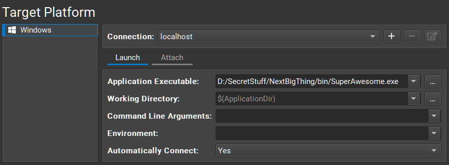
First, set up a connection to the app to be profiled. Choose Connect and fill in the required parameters for launching your game (Figure 1).

Screenshot includes fields for the path to the application executable, working directory, command-line arguments, and so on.
Figure 1. Connection settings

Select GPU Trace as the activity, with Metric Set configured to Advanced Mode Metrics. Using Advanced Mode Metrics requires a stable and consistent frame, because the analysis runs over several passes over several frames. If your application doesn’t meet these requirements, you can use the Nsight Graphics built-in C++ Capture tool to capture a frame of your application and create a new EXE that replays the same frame repeatedly.

Choose Launch GPU Trace to launch your application. When you reach a frame that you’d like to capture, choose Generate GPU Trace Capture or press F11.

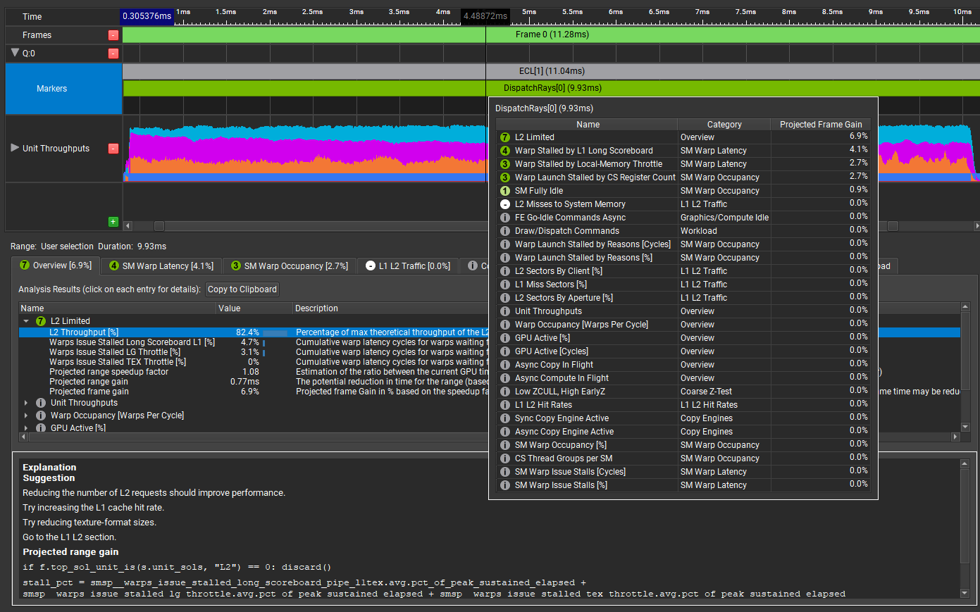
When the capture is complete, stop the application and open the trace. Choose Trace Analysis. In the Analysis panel of GPU Trace (Figure 2), double-click or hover over the marker for the range to analyze, in this case, DispatchRays[0]:

Screenshot of the Trace Analysis results with a large tooltip overlay.
Figure 2. Trace Analysis results

The tooltip presents a compact view of all performance gain opportunities that the tool has detected in this GPU workload, sorted by their projected GPU frame-time gain. The workload has the following limiters:

  • L2 Limited: Being L2 limited might be indicative of a problem. With knowledge of the workload, it’s not necessarily something that you would expect.
  • Warp Stalled by L1 Long Scoreboard: This is a common reason for warps to be stalled, often due to texture fetches. If there is not enough work between a texture lookup being initiated and the result of the lookup being used, then the warp is stalled until the texture lookup is satisfied.
  • Warp Stalled by Local-Memory Throttle: Local memory is ‘thread local’. It’s memory that is local to each thread, as opposed to group-shared memory that is shared between all the threads in the thread group.  It’s unusual for a shader to need any local memory, so this is interesting. And what does local-memory throttling mean? There’s more to learn here.

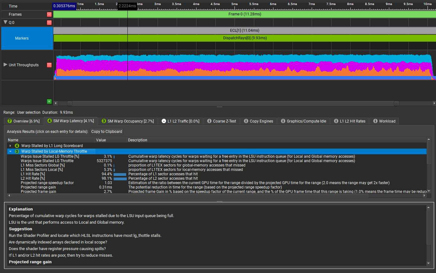
Choose SM Warp Latency and Warp Stalled by Local-Memory Throttle.

The Trace Analysis view, showing an explanation of whatever is selected in the analysis results; in this case, an explanation of Local Memory Throttle.
Figure 3. Trace Analysis explanation of Local Memory Throttle

The Explanation window gives a more meaningful description of the problem, with some helpful suggestions. It suggests launching the Shader Profiler to locate the specific HLSL instructions that have lg_throttle stalls.

Step 2: Switch to the Shader Profiler

Before you use the Shader Profiler, it’s important to make sure that Nsight Graphics can get access to symbols for your shaders. The easiest way to achieve this is to make sure that the shaders are compiled with the /Zi option, and embed the symbols in the shader binary.

Sometimes it’s preferable to configure the compilation so that the symbols go into an external PDB file. In that case, be sure to specify the correct path under Tools, Options.

When Nsight Graphics can see the shader symbols, it can map locations in the shader back to the source code, which makes it far easier for you to tell what’s going on. If Nsight Graphics doesn’t have access to symbols, then you can only see the shader disassembly (for example, DXIL).

The Shader Profiler is part of the Frame Profiler. Connect to the application again but this time, choose Frame Profiler under Activity. When you choose Launch Frame Profiler, the application should launch with this HUD (Figure 4) on top of it.

Profiler overlay, showing the request to press F11 to capture a frame.
Figure 4. Profiler overlay

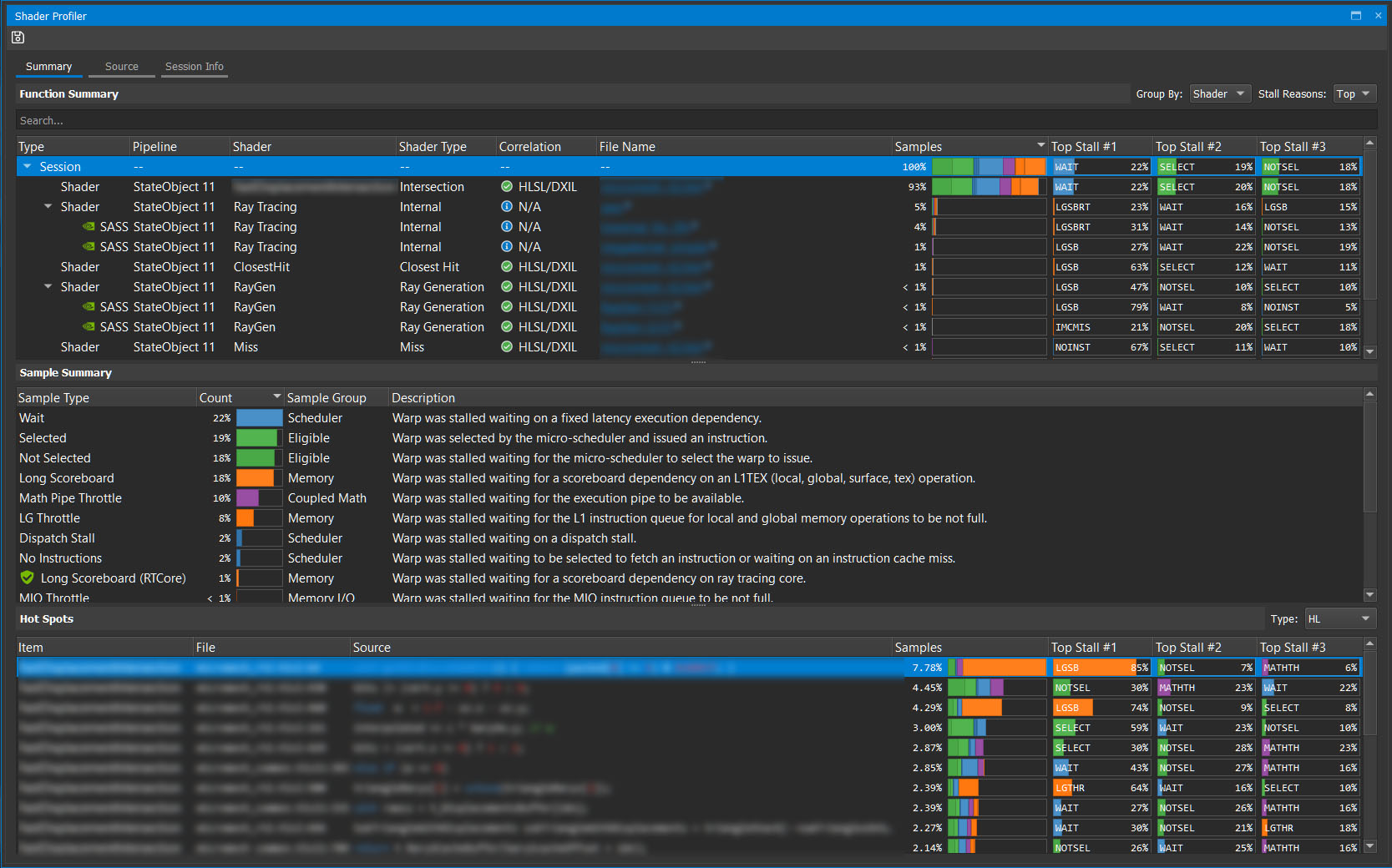
Navigate to the part of the application to profile and press F11 to capture a frame for analysis. From here, choose Profile Shaders in Nsight Graphics. This runs a short sampling session, and then presents you with a summary view (Figure 5).

The Shader Profiler view, showing a summary of hotspots sorted by sample count.
Figure 5. Shader Profiler summary view

Here’s a breakdown.

The Function Summary shows a list of the top shaders, in order of the number of samples that hit in those shaders. This is a good proxy for the shader latency and lets you concentrate on the shaders that can yield the biggest benefit from optimizing.

In the Correlation column, there are multiple green ticks, which are always good. In this case, it means that Nsight Graphics has been able to correlate the samples back to the source code.

To open up the shader view, select the first file name. On the left is the source code, and on the right is DXIL. For the purposes of this post, you don’t have to care about the DXIL, so change the view to just HLSL

It’s quite subtle, but there’s an important heat map of instruction samples on the far right, just to the right of the scroll bar. Remember, GPU Trace Analysis suggested that you should look for lg_throttle stalls. It said:

LSU is the unit that performs access to Local and Global memory.
Run the Shader Profiler and locate which HLSL instructions have most lg_thottle stalls.
Are dynamically indexed arrays declared in local scope?
Does the shader have register pressure causing spills?
If L1 and L2 hit rates are poor, then try to reduce misses.

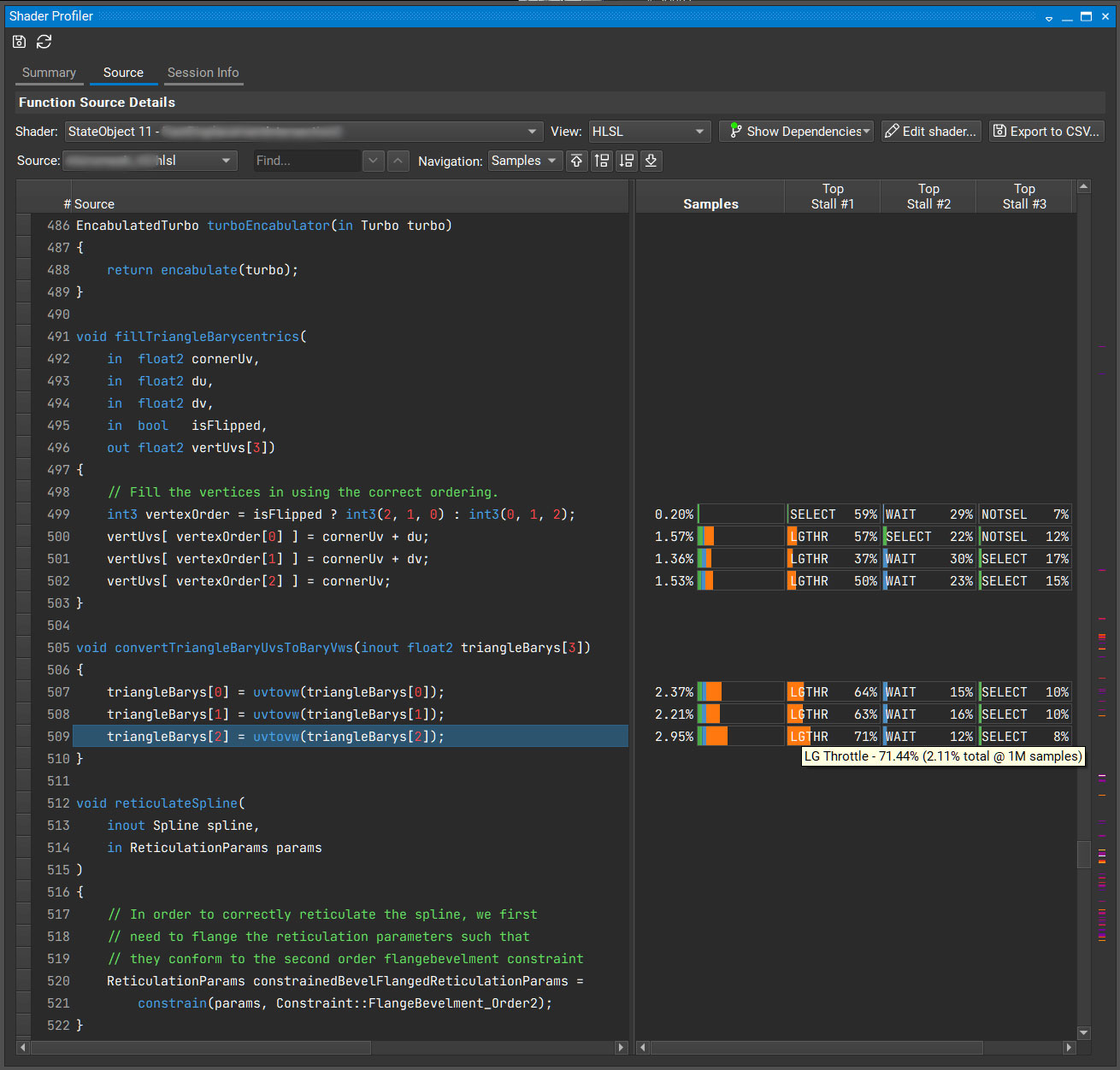
In the Shader Profiler, the samples that show as LGTHR are stalled due to lg_throttle reasons.

Shader Profiler source view, split into left and right panes. (left) The shader source code. (right) Sample counts and a breakdown of the stall reasons with each sample.
Figure 6. Shader Profiler source view with samples and stall reasons

“Are dynamically indexed arrays declared in local scope?”

Dynamically indexed arrays are indexed by a variable, where the value of the index is not known at compile time.

When this happens, the compiler often puts the array in local memory instead of it living in registers. Memory is slower than registers.

The following code example shows a dynamically indexed array.

vertUvs[vertexOrder[0]] = cornerUv + du;
vertUvs[vertexOrder[1]] = cornerUv + dv;
vertUvs[vertexOrder[2]] = cornerUv;

What’s going on? It looks like the code fills in the array in a different order, depending on whether the triangle is flipped.

int3 vertexOrder = isFlipped ? int3(2, 1, 0) : int3(0, 1, 2);

The act of dynamically indexing this array makes the compiler move this array into memory. It affects this bit of code and all the bits of code that reference that array. That’s why convertTriangleBaryUvsToBaryVws is showing up as hot, too.

Can you do this without dynamic indexing? Yes, you can. Changing how the flip is done results in Figure 7.

Screenshot of alternative code using a branch instead of dynamic indexing.
Figure 7. Alternative code not using dynamic indexing

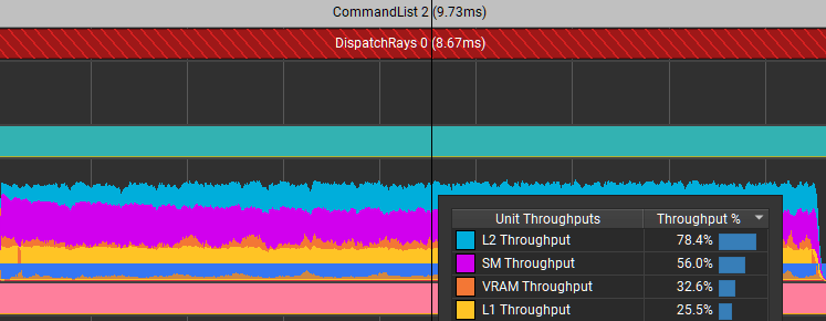
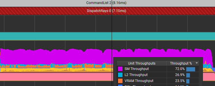
Those particular stalls are eliminated. It reduced the time for this dispatch from 8.67 ms down to 7.1 ms. Not only did it improve the efficiency of shader code, but it also massively reduced the limiter in L2 because of the reduced memory traffic.

Before optimization, DispatchRays takes 8.67 ms.
Figure 8. Trace before optimization
After optimization, DispatchRays takes 7.1 ms.
Figure 9. Trace after optimization

Summary

NVIDIA Nsight Graphics is a powerful tool for analyzing your rendering workloads. This has been a quick walkthrough, just touching on some capabilities. We highly recommend using it.

Disclaimer

The tests and results in this post were true as of driver version 467.07. Driver and compiler development continues all the time. That means that optimization opportunities can change over time too.

Categories
Misc

Relevant point on an image – where to start?

Bit of a newbie to TF/the machine learning world. I’ve built/trained image classification & segmentation models before and have tinkered with TF recommenders before. My knowledge probably doesn’t go beyond the first few layers of the documentation/tutorials, though.

I’m wondering as to how I might accomplish something along these lines: I have approximately 20,000 images and I have manually placed a simple text watermark over the image to partially cover the subject of the image (the subject takes up 80% of the image and the watermark takes up approx 5% of the image), the watermark is small and subtle, only really noticeable if you zoom in. I have saved the coordinates for each watermark for each image file. I’m now looking to automate the placing of watermarks in a subtle position on the subject.

Could someone please link to some documentation/guides which would be appropriate for training a model to achieve this goal? I am assuming I need something along the lines of image classification but a lot of what I’m seeing is that it’s just for classifying what’s in an image/segmenting (drawing a box) around an object in the image rather than saying “given this image, this particular point on the subject in the image is relevant”.

MTIA

submitted by /u/IcyFish0
[visit reddit] [comments]

Categories
Offsites

Google at ICLR 2022

The 10th International Conference on Learning Representations (ICLR 2022) kicks off this week, bringing together researchers, entrepreneurs, engineers and students alike to discuss and explore the rapidly advancing field of deep learning. Entirely virtual this year, ICLR 2022 offers conference and workshop tracks that present some of the latest research in deep learning and its applications to areas ranging from computer vision, speech recognition and text understanding to robotics, computational biology, and more.

As a Platinum Sponsor of ICLR 2022 and Champion DEI Action Fund contributor, Google will have a robust presence with nearly 100 accepted publications and extensive participation on organizing committees and in workshops. If you have registered for ICLR 2022, we hope you’ll watch our talks and learn about the work done at Google to address complex problems that affect billions of people. Here you can learn more about the research we will be presenting as well as our general involvement at ICLR 2022 (those with Google affiliations in bold).

Senior Area Chairs:
Includes: Been Kim, Dale Schuurmans, Sergey Levine

Area Chairs:
Includes: Adam White, Aditya Menon, Aleksandra Faust, Amin Karbasi, Amir Globerson, Andrew Dai, Balaji Lakshminarayanan, Behnam Neyshabur, Ben Poole, Bhuwan Dhingra, Bo Dai, Boqing Gong, Cristian Sminchisescu, David Ha, David Woodruff, Denny Zhou, Dipanjan Das, Dumitru Erhan, Dustin Tran, Emma Strubell, Eunsol Choi, George Dahl, George Tucker, Hanie Sedghi, Heinrich Jiang, Hossein Mobahi, Hugo Larochelle, Izhak Shafran, Jasper Snoek, Jean-Philippe Vert, Jeffrey Pennington, Justin Gilmer, Karol Hausman, Kevin Swersky, Krzysztof Choromanski, Mathieu Blondel, Matt Kusner, Michael Ryoo, Ming-Hsuan Yang, Minmin Chen, Mirella Lapata, Mohammad Ghavamzadeh, Mohammad Norouzi, Naman Agarwal, Nicholas Carlini, Olivier Bachem, Piyush Rai, Prateek Jain, Quentin Berthet, Richard Nock, Rose Yu, Sewoong Oh, Silvio Lattanzi, Slav Petrov, Srinadh Bhojanapalli, Tim Salimans, Ting Chen, Tong Zhang, Vikas Sindhwani, Weiran Wang, William Cohen, Xiaoming Liu

Workflow Chairs:
Includes: Yaguang Li

Diversity Equity & Inclusion Chairs:
Includes: Rosanne Liu

Invited Talks
Beyond Interpretability: Developing a Language to Shape Our Relationships with AI
Google Speaker: Been Kim

Do You See What I See? Large-Scale Learning from Multimodal Videos
Google Speaker: Cordelia Schmid

Publications
Hyperparameter Tuning with Renyi Differential Privacy – 2022 Outstanding Paper Award
Nicolas Papernot, Thomas Steinke

MIDI-DDSP: Detailed Control of Musical Performance via Hierarchical Modeling
Yusong Wu, Ethan Manilow, Yi Deng, Rigel Swavely, Kyle Kastner, Tim Cooijmans, Aaron Courville, Cheng-Zhi Anna Huang, Jesse Engel

The Information Geometry of Unsupervised Reinforcement Learning
Benjamin Eysenbach, Ruslan Salakhutdinov, Sergey Levine

Learning Strides in Convolutional Neural Networks – 2022 Outstanding Paper Award
Rachid Riad*, Olivier Teboul, David Grangier, Neil Zeghidour

Poisoning and Backdooring Contrastive Learning
Nicholas Carlini, Andreas Terzis

Coordination Among Neural Modules Through a Shared Global Workspace
Anirudh Goyal, Aniket Didolkar, Alex Lamb, Kartikeya Badola, Nan Rosemary Ke, Nasim Rahaman, Jonathan Binas, Charles Blundell, Michael Mozer, Yoshua Bengio

Fine-Tuned Language Models Are Zero-Shot Learners (see the blog post)
Jason Wei, Maarten Bosma, Vincent Y. Zhao, Kelvin Guu, Adams Wei Yu, Brian Lester, Nan Du, Andrew M. Dai, Quoc V. Le

Large Language Models Can Be Strong Differentially Private Learners
Xuechen Li, Florian Tramèr, Percy Liang, Tatsunori Hashimoto

Progressive Distillation for Fast Sampling of Diffusion Models
Tim Salimans, Jonathan Ho

Exploring the Limits of Large Scale Pre-training
Samira Abnar, Mostafa Dehghani, Behnam Neyshabur, Hanie Sedghi

Scarf: Self-Supervised Contrastive Learning Using Random Feature Corruption
Dara Bahri, Heinrich Jiang, Yi Tay, Donald Metzler

Scalable Sampling for Nonsymmetric Determinantal Point Processes
Insu Han, Mike Gartrell, Jennifer Gillenwater, Elvis Dohmatob, Amin Karbasi

When Vision Transformers Outperform ResNets without Pre-training or Strong Data Augmentations
Xiangning Chen, Cho-Jui Hsieh, Boqing Gong

ViTGAN: Training GANs with Vision Transformers
Kwonjoon Lee, Huiwen Chang, Lu Jiang, Han Zhang, Zhuowen Tu, Ce Liu

Generalized Decision Transformer for Offline Hindsight Information Matching
Hiroki Furuta, Yutaka Matsuo, Shixiang Shane Gu

The MultiBERTs: BERT Reproductions for Robustness Analysis
Thibault Sellam, Steve Yadlowsky, Ian Tenney, Jason Wei, Naomi Saphra, Alexander D’Amour, Tal Linzen, Jasmijn Bastings, Iulia Turc, Jacob Eisenstein, Dipanjan Das, Ellie Pavlick

Scaling Laws for Neural Machine Translation
Behrooz Ghorbani, Orhan Firat, Markus Freitag, Ankur Bapna, Maxim Krikun, Xavier Garcia, Ciprian Chelba, Colin Cherry

Interpretable Unsupervised Diversity Denoising and Artefact Removal
Mangal Prakash, Mauricio Delbracio, Peyman Milanfar, Florian Jug

Understanding Latent Correlation-Based Multiview Learning and Self-Supervision: An Identifiability Perspective
Qi Lyu, Xiao Fu, Weiran Wang, Songtao Lu

Memorizing Transformers
Yuhuai Wu, Markus N. Rabe, DeLesley Hutchins, Christian Szegedy

Churn Reduction via Distillation
Heinrich Jiang, Harikrishna Narasimhan, Dara Bahri, Andrew Cotter, Afshin Rostamizadeh

DR3: Value-Based Deep Reinforcement Learning Requires Explicit Regularization
Aviral Kumar, Rishabh Agarwal, Tengyu Ma, Aaron Courville, George Tucker, Sergey Levine

Path Auxiliary Proposal for MCMC in Discrete Space
Haoran Sun, Hanjun Dai, Wei Xia, Arun Ramamurthy

On the Relation Between Statistical Learning and Perceptual Distances
Alexander Hepburn, Valero Laparra, Raul Santos-Rodriguez, Johannes Ballé, Jesús Malo

Possibility Before Utility: Learning And Using Hierarchical Affordances
Robby Costales, Shariq Iqbal, Fei Sha

MT3: Multi-Task Multitrack Music Transcription
Josh Gardner*, Ian Simon, Ethan Manilow*, Curtis Hawthorne, Jesse Engel

Bayesian Neural Network Priors Revisited
Vincent Fortuin, Adrià Garriga-Alonso, Sebastian W. Ober, Florian Wenzel, Gunnar Rätsch, Richard E. Turner, Mark van der Wilk, Laurence Aitchison

GradMax: Growing Neural Networks using Gradient Information
Utku Evci, Bart van Merrienboer, Thomas Unterthiner, Fabian Pedregosa, Max Vladymyrov

Scene Transformer: A Unified Architecture for Predicting Future Trajectories of Multiple Agents
Jiquan Ngiam, Benjamin Caine, Vijay Vasudevan, Zhengdong Zhang, Hao-Tien Lewis Chiang, Jeffrey Ling, Rebecca Roelofs, Alex Bewley, Chenxi Liu, Ashish Venugopal, David Weiss, Ben Sapp, Zhifeng Chen, Jonathon Shlens

The Role of Pretrained Representations for the OOD Generalization of RL Agents
Frederik Träuble, Andrea Dittadi, Manuel Wüthrich, Felix Widmaier, Peter Gehler, Ole Winther, Francesco Locatello, Olivier Bachem, Bernhard Schölkopf, Stefan Bauer

Autoregressive Diffusion Models
Emiel Hoogeboom, Alexey A. Gritsenko, Jasmijn Bastings, Ben Poole, Rianne van den Berg, Tim Salimans

The Role of Permutation Invariance in Linear Mode Connectivity of Neural Networks
Rahim Entezari, Hanie Seghi, Olga Saukh, Behnam Neyshabur

DISSECT: Disentangled Simultaneous Explanations via Concept Traversals
Asma Ghandeharioun, Been Kim, Chun-Liang Li, Brendan Jou, Brian Eoff, Rosalind W. Picard

Anisotropic Random Feature Regression in High Dimensions
Gabriel C. Mel, Jeffrey Pennington

Open-Vocabulary Object Detection via Vision and Language Knowledge Distillation
Xiuye Gu, Tsung-Yi Lin*, Weicheng Kuo, Yin Cui

MCMC Should Mix: Learning Energy-Based Model with Flow-Based Backbone
Erik Nijkamp*, Ruiqi Gao, Pavel Sountsov, Srinivas Vasudevan, Bo Pang, Song-Chun Zhu, Ying Nian Wu

Effect of Scale on Catastrophic Forgetting in Neural Networks
Vinay Ramasesh, Aitor Lewkowycz, Ethan Dyer

Incremental False Negative Detection for Contrastive Learning
Tsai-Shien Chen, Wei-Chih Hung, Hung-Yu Tseng, Shao-Yi Chien, Ming-Hsuan Yang

Towards Evaluating the Robustness of Neural Networks Learned by Transduction
Jiefeng Chen, Xi Wu, Yang Guo, Yingyu Liang, Somesh Jha

What Do We Mean by Generalization in Federated Learning?
Honglin Yuan*, Warren Morningstar, Lin Ning, Karan Singhal

ViDT: An Efficient and Effective Fully Transformer-Based Object Detector
Hwanjun Song, Deqing Sun, Sanghyuk Chun, Varun Jampani, Dongyoon Han, Byeongho Heo, Wonjae Kim, Ming-Hsuan Yang

Measuring CLEVRness: Black-Box Testing of Visual Reasoning Models
Spyridon Mouselinos, Henryk Michalewski, Mateusz Malinowski

Wisdom of Committees: An Overlooked Approach To Faster and More Accurate Models (see the blog post)
Xiaofang Wang, Dan Kondratyuk, Eric Christiansen, Kris M. Kitani, Yair Alon (prev. Movshovitz-Attias), Elad Eban

Leveraging Unlabeled Data to Predict Out-of-Distribution Performance
Saurabh Garg*, Sivaraman Balakrishnan, Zachary C. Lipton, Behnam Neyshabur, Hanie Sedghi

Data-Driven Offline Optimization for Architecting Hardware Accelerators (see the blog post)
Aviral Kumar, Amir Yazdanbakhsh, Milad Hashemi, Kevin Swersky, Sergey Levine

Diurnal or Nocturnal? Federated Learning of Multi-branch Networks from Periodically Shifting Distributions
Chen Zhu*, Zheng Xu, Mingqing Chen, Jakub Konecny, Andrew Hard, Tom Goldstein

Policy Gradients Incorporating the Future
David Venuto, Elaine Lau, Doina Precup, Ofir Nachum

Discrete Representations Strengthen Vision Transformer Robustness
Chengzhi Mao*, Lu Jiang, Mostafa Dehghani, Carl Vondrick, Rahul Sukthankar, Irfan Essa

SimVLM: Simple Visual Language Model Pretraining with Weak Supervision (see the blog post)
Zirui Wang, Jiahui Yu, Adams Wei Yu, Zihang Dai, Yulia Tsvetkov, Yuan Cao

Neural Stochastic Dual Dynamic Programming
Hanjun Dai, Yuan Xue, Zia Syed, Dale Schuurmans, Bo Dai

PolyLoss: A Polynomial Expansion Perspective of Classification Loss Functions
Zhaoqi Leng, Mingxing Tan, Chenxi Liu, Ekin Dogus Cubuk, Xiaojie Shi, Shuyang Cheng, Dragomir Anguelov

Information Prioritization Through Empowerment in Visual Model-Based RL
Homanga Bharadhwaj*, Mohammad Babaeizadeh, Dumitru Erhan, Sergey Levine

Value Function Spaces: Skill-Centric State Abstractions for Long-Horizon Reasoning
Dhruv Shah, Peng Xu, Yao Lu, Ted Xiao, Alexander Toshev, Sergey Levine, Brian Ichter

Understanding and Leveraging Overparameterization in Recursive Value Estimation
Chenjun Xiao, Bo Dai, Jincheng Mei, Oscar Ramirez, Ramki Gummadi, Chris Harris, Dale Schuurmans

The Efficiency Misnomer
Mostafa Dehghani, Anurag Arnab, Lucas Beyer, Ashish Vaswani, Yi Tay

On the Role of Population Heterogeneity in Emergent Communication
Mathieu Rita, Florian Strub, Jean-Bastien Grill, Olivier Pietquin, Emmanuel Dupoux

No One Representation to Rule Them All: Overlapping Features of Training Methods
Raphael Gontijo-Lopes, Yann Dauphin, Ekin D. Cubuk

Data Poisoning Won’t Save You From Facial Recognition
Evani Radiya-Dixit, Sanghyun Hong, Nicholas Carlini, Florian Tramèr

AdaMatch: A Unified Approach to Semi-Supervised Learning and Domain Adaptation
David Berthelot, Rebecca Roelofs, Kihyuk Sohn, Nicholas Carlini, Alex Kurakin

Maximum Entropy RL (Provably) Solves Some Robust RL Problems
Benjamin Eysenbach, Sergey Levine

Auto-scaling Vision Transformers Without Training
Wuyang Chen, Wei Huang, Xianzhi Du, Xiaodan Song, Zhangyang Wang, Denny Zhou

Optimizing Few-Step Diffusion Samplers by Gradient Descent
Daniel Watson, William Chan, Jonathan Ho, Mohammad Norouzi

ExT5: Towards Extreme Multi-Task Scaling for Transfer Learning
Vamsi Aribandi, Yi Tay, Tal Schuster, Jinfeng Rao, Huaixiu Steven Zheng, Sanket Vaibhav Mehta, Honglei Zhuang, Vinh Q. Tran, Dara Bahri, Jianmo Ni, Jai Gupta, Kai Hui, Sebastian Ruder, Donald Metzler

Fortuitous Forgetting in Connectionist Networks
Hattie Zhou, Ankit Vani, Hugo Larochelle, Aaron Courville

Evading Adversarial Example Detection Defenses with Orthogonal Projected Gradient Descent
Oliver Bryniarski, Nabeel Hingun, Pedro Pachuca, Vincent Wang, Nicholas Carlini

Benchmarking the Spectrum of Agent Capabilities
Danijar Hafner

Charformer: Fast Character Transformers via Gradient-Based Subword Tokenization
Yi Tay, Vinh Q. Tran, Sebastian Ruder, Jai Gupta, Hyung Won Chung, Dara Bahri, Zhen Qin, Simon Baumgartner, Cong Yu, Donald Metzler

Mention Memory: Incorporating Textual Knowledge into Transformers Through Entity Mention Attention
Michiel de Jong, Yury Zemlyanskiy, Nicholas FitzGerald, Fei Sha, William Cohen

Eigencurve: Optimal Learning Rate Schedule for SGD on Quadratic Objectives with Skewed Hessian Spectrums
Rui Pan, Haishan Ye, Tong Zhang

Scale Efficiently: Insights from Pre-training and Fine-Tuning Transformers
Yi Tay, Mostafa Dehghani, Jinfeng Rao, William Fedus, Samira Abnar, Hyung Won Chung, Sharan Narang, Dani Yogatama, Ashish Vaswani, Donald Metzler

Omni-Scale CNNs: A Simple and Effective Kernel Size Configuration for Time Series Classification
Wensi Tang, Guodong Long, Lu Liu,Tianyi Zhou, Michael Blumenstein, Jing Jiang

Embedded-Model Flows: Combining the Inductive Biases of Model-Free Deep Learning and Explicit Probabilistic Modeling
Gianluigi Silvestri, Emily Fertig, Dave Moore, Luca Ambrogioni

Post Hoc Explanations May be Ineffective for Detecting Unknown Spurious Correlation
Julius Adebayo, Michael Muelly, Hal Abelson, Been Kim

Axiomatic Explanations for Visual Search, Retrieval, and Similarity Learning
Mark Hamilton, Scott Lundberg, Stephanie Fu, Lei Zhang, William T. Freeman

Pix2seq: A Language Modeling Framework for Object Detection (see the blog post)
Ting Chen, Saurabh Saxena, Lala Li, David J. Fleet, Geoffrey Hinton

Mirror Descent Policy Optimization
Manan Tomar, Lior Shani, Yonathan Efroni, Mohammad Ghavamzadeh

CodeTrek: Flexible Modeling of Code Using an Extensible Relational Representation
Pardis Pashakhanloo, Aaditya Naik, Yuepeng Wang, Hanjun Dai, Petros Maniatis, Mayur Naik

Conditional Object-Centric Learning From Video
Thomas Kipf, Gamaleldin F. Elsayed, Aravindh Mahendran, Austin Stone, Sara Sabour, Georg Heigold, Rico Jonschkowski, Alexey Dosovitskiy, Klaus Greff

A Loss Curvature Perspective on Training Instabilities of Deep Learning Models
Justin Gilmer, Behrooz Ghorbani, Ankush Garg, Sneha Kudugunta, Behnam Neyshabur, David Cardoze, George E. Dahl, Zack Nado, Orhan Firat

Autonomous Reinforcement Learning: Formalism and Benchmarking
Archit Sharma, Kelvin Xu, Nikhil Sardana, Abhishek Gupta, Karol Hausman, Sergey Levine, Chelsea Finn

TRAIL: Near-Optimal Imitation Learning with Suboptimal Data
Mengjiao Yang, Sergey Levine, Ofir Nachum

Minimax Optimization With Smooth Algorithmic Adversaries
Tanner Fiez, Lillian J. Ratliff, Chi Jin, Praneeth Netrapalli

Unsupervised Semantic Segmentation by Distilling Feature Correspondences
Mark Hamilton, Zhoutong Zhang, Bharath Hariharan, Noah Snavely, William T. Freeman

InfinityGAN: Towards Infinite-Pixel Image Synthesis
Chieh Hubert Lin, Hsin-Ying Lee, Yen-Chi Cheng, Sergey Tulyakov, Ming-Hsuan Yang

Shuffle Private Stochastic Convex Optimization
Albert Cheu, Matthew Joseph, Jieming Mao, Binghui Peng

Hybrid Random Features
Krzysztof Choromanski, Haoxian Chen, Han Lin, Yuanzhe Ma, Arijit Sehanobish, Deepali Jain, Michael S Ryoo, Jake Varley, Andy Zeng, Valerii Likhosherstov, Dmitry Kalashnikov, Vikas Sindhwani, Adrian Weller

Vector-Quantized Image Modeling With Improved VQGAN
Jiahui Yu, Xin Li, Jing Yu Koh, Han Zhang, Ruoming Pang, James Qin, Alexander Ku, Yuanzhong Xu, Jason Baldridge, Yonghui Wu

On the Benefits of Maximum Likelihood Estimation for Regression and Forecasting
Pranjal Awasthi, Abhimanyu Das, Rajat Sen, Ananda Theertha Suresh

Surrogate Gap Minimization Improves Sharpness-Aware Training
Juntang Zhuang*, Boqing Gong, Liangzhe Yuan, Yin Cui, Hartwig Adam, Nicha C. Dvornek, Sekhar Tatikonda, James S. Duncan, Ting Liu

Online Target Q-learning With Reverse Experience Replay: Efficiently Finding the Optimal Policy for Linear MDPs
Naman Agarwal, Prateek Jain, Dheeraj Nagaraj, Praneeth Netrapalli, Syomantak Chaudhuri

CrossBeam: Learning to Search in Bottom-Up Program Synthesis
Kensen Shi, Hanjun Dai, Kevin Ellis, Charles Sutton

Workshops
Workshop on the Elements of Reasoning: Objects, Structure, and Causality (OSC)
Organizers include: Klaus Greff, Thomas Kipf

Workshop on Agent Learning in Open-Endedness
Organizers include: Krishna Srinivasan
Speakers include: Natasha Jaques, Danijar Hafner

Wiki-M3L: Wikipedia and Multi-modal & Multi-lingual Research
Organizers include: Klaus Greff, Thomas Kipf
Speakers include: Jason Baldridge, Tom Duerig

Setting Up ML Evaluation Standards to Accelerate Progress
Organizers include: Rishabh Agarwal
Speakers and Panelists include: Katherine Heller, Sara Hooker, Corinna Cortes

From Cells to Societies: Collective Learning Across Scales
Organizers include: Mark Sandler, Max Vladymyrov
Speakers include: Blaise Aguera y Arcas, Alexander Mordvintsev, Michael Mozer

Emergent Communication: New Frontiers
Speakers include: Natasha Jaques

Deep Learning for Code
Organizers include: Jonathan Herzig

GroundedML: Anchoring Machine Learning in Classical Algorithmic Theory
Speakers include: Gintare Karolina Dziugaite

Generalizable Policy Learning in the Physical World
Speakers and Panelists include: Mrinal Kalakrishnan

CoSubmitting Summer (CSS) Workshop
Organizers include: Rosanne Liu


*Work done while at Google.